Greedy Algorithm: A Beginner’s Guide
In a recent study published by ACM Transactions on Mathematical Software, researchers have analyzed the performance of greedy algorithms on a set of 200 optimization problems. They concluded that greedy algorithms found the optimal solution for 52% of the problems. A different study compared greedy algorithms to other types on 100 optimization problems. As published in Operations Research Letters, they found that greedy algorithms were the most efficient algorithms for 60% of the problems. This sums up the importance of the Greedy algorithm.
Table of Contents
- What is a Greedy Algorithm?
- How Do Greedy Algorithms Work?
- Greedy Algorithm Vs. Divide and Conquer Algorithm
- Applications of Greedy Algorithms
- Advantages of Greedy Algorithms
- What are the Drawbacks of the Greedy Algorithm?
- Examples of Greedy Algorithms
- Conclusion
Kickstart your coding journey through our YouTube channel on
{
“@context”: “https://schema.org”,
“@type”: “VideoObject”,
“name”: “C Tutorial for Beginners | C Programming Tutorial | Intellipaat”,
“description”: “Greedy Algorithm: A Beginner’s Guide”,
“thumbnailUrl”: “https://img.youtube.com/vi/T3MusSv2zBQ/hqdefault.jpg”,
“uploadDate”: “2023-09-05T08:00:00+08:00”,
“publisher”: {
“@type”: “Organization”,
“name”: “Intellipaat Software Solutions Pvt Ltd”,
“logo”: {
“@type”: “ImageObject”,
“url”: “https://intellipaat.com/blog/wp-content/themes/intellipaat-blog-new/images/logo.png”,
“width”: 124,
“height”: 43
}
},
“embedUrl”: “https://www.youtube.com/embed/T3MusSv2zBQ”
}
What is a Greedy Algorithm?

A greedy algorithm is an algorithmic paradigm that makes a series of choices by consistently selecting the most immediate or obvious opportunity to optimize a desired objective. The hallmark of a greedy algorithm is its snap decision-making process, where each decision is based on the assumption that a sequence of locally optimal solutions might lead to a globally optimal solution.
Let’s understand it by a real-life example, Imagine a child in a room filled with candy jars. Each jar has a label showing how many candies are inside. The child has limited time to leave the room. The child wants to collect as many candies as possible in the short time they have.
The term “greedy algorithm” originates from how the method makes the best choice at each stage. To be precise, the origin of the term is not attributed to a singular individual. However, the foundations of greedy principles can be traced back to various optimization problems tackled during the mid-20th century. One of the most classic applications of the greedy approach is Kruskal’s and Prim’s algorithms for finding the minimum spanning tree of a graph.
Greedy algorithms have been applied across a wide array of problems, from job scheduling and Huffman coding to fractional knapsack and coin change problems. Its simplicity and often efficient results have made it a popular choice among problem solvers. However, it is noteworthy that while greedy algorithms work well for certain problems, they don’t always guarantee the best solution for every problem due to their local optimization nature.
In recent times, with the explosion of data and complex computational problems, the greedy approach has been combined with other algorithmic paradigms or used as a heuristic in more sophisticated methods. This allows for utilizing the simplicity of the greedy method while offsetting its limitations.
Enroll in our C programming course to add a new skill to your skills bucket.
What are the Components of the Greedy Algorithm?
The greedy algorithm, known for its efficiency in problem-solving within computational domains, uses a strategic approach to achieve locally optimal solutions. This method’s modus operandi is directed by a set of principal components, each playing a key role in steering the algorithm toward its intended solution.
The greedy algorithm’s efficacy can be attributed to five cardinal components, which collectively navigate the problem-solving journey from initiation to completion.
The following describes these integral components:
- Candidate Set: It refers to the initial set of potential solutions from which the algorithm can select. Every potential element that could become part of the final solution is contained within this set. The algorithm progresses by inspecting and evaluating these candidates.
- Selection Function: It acts as the algorithm’s discerning eye. The selection function evaluates candidates from the candidate set. This function determines which candidate is most favorable or promising at a given iteration based on specific criteria. The selected candidate is then added to the partial solution, paving the way for the next decision-making step.
- Feasibility Function: Every selected candidate must undergo a validation check, ensuring it can be feasibly incorporated into the existing partial solution without violating any constraints. The feasibility function performs this check, ascertaining if the inclusion of a candidate maintains the integrity of the solution-in-progress.
- Objective Function: The objective function provides a metric to evaluate the quality or desirability of a solution. It quantifies how ‘good’ a solution is, determining whether one solution is more optimal than another. In the context of the greedy algorithm, this function often measures the local optimality of solutions.
- Solution Function: After iterative selections and evaluations, the algorithm must determine when an optimal or satisfactory solution has been achieved. The solution function dictates when the algorithm can stop, marking the point where further additions to the solution would no longer be beneficial or possible.
When to Use a Greedy Algorithm

The greedy algorithm is known for being efficient. It chooses the best option at each step to find the best overall outcome.
But when exactly should one employ this approach?
- Optimal Substructure: The greedy algorithm works best for problems that can be broken down into smaller parts. Making a good choice locally also leads to the best solution overall. For instance, problems like the Minimum Spanning Tree exhibit this trait.
- No Future Constraints: The greedy algorithm works best when current decisions don’t limit future choices. If the current choice doesn’t affect decisions that will be made later, the algorithm can operate effectively.
- Incremental Solution: When the solution can be built step by step, often by picking from a sorted list, the greedy approach is very effective. Problems such as fractional knapsack and job scheduling are classic examples.
- Simplicity and Efficiency: The greedy algorithm is a good choice when you need a fast solution. It’s simple and works well when exact optimization takes too long.
Learn more about computer programming through our C programming tutorial for absolute beginners.
How Do Greedy Algorithms Work?
As the name suggests, greedy algorithms operate by making the most beneficial choice at each decision-making step. This ‘greedy’ approach ensures that the algorithm seeks local optimality, hoping that such local decisions will lead to a globally optimal solution.
Let’s understand the Greedy approach with a real-life example:
The Coin Change Problem: Consider a cashier tasked with giving change to a customer. The cashier has denominations of 25 cents (quarters), 10 cents (dimes), 5 cents (nickels), and 1 cent (pennies). The goal is to provide the least number of coins that sum up to a given amount.
Let’s break this down:
Imagine a customer overpaying by 93 cents. A naive approach would involve the cashier giving out 93 pennies. But that’s inefficient. Instead, a more intuitive or ‘greedy’, approach would be to give the largest possible coin denomination first and continue doing so until the entire amount is paid.
- First Step: 93 cents: The largest denomination less than 93 is a quarter (25 cents).
Hand out a quarter
Remaining amount = 68 cents - Second Step: 68 cents: Again, give out a quarter.
Remaining amount = 43 cents - Third Step: 43 cents: Yet again, another quarter
Remaining amount = 18 cents - Fourth Step: 18 cents: This time, a dime fits the bill.
Remaining amount = 8 cents - Fifth Step: 8 cents: Two pennies after a nickel
Remaining amount = 0 cents
In just five coins (three quarters, one dime, one nickel, and two pennies), the cashier has efficiently provided the change. This is the essence of a greedy algorithm. At every step, the algorithm makes the most optimal decision without thinking about future consequences.
Such is the power and elegance of the greedy algorithm. A method that doesn’t forecast the entirety of future outcomes but marches forward, making the best immediate decision, much like the cashier minimizing the coin count.
Now, we have a glimpse of the workings of the greedy algorithm. Moving forward, let’s see how the greedy algorithm is implemented in code.
Initialize solution set S to empty
While the solution is not complete:
   Choose the best candidate from candidate set C
   If candidate is feasible:
       Add the candidate to solution set S
   Remove the chosen candidate from C
Return solution set S
Problem statement: Write a program to show the implementation of the greedy algorithm.
#include
using namespace std;
vector greedyAlgorithm(vector &candidates) {
    vector solution;
    while(!candidates.empty()) {
        int best_candidate = *max_element(candidates.begin(), candidates.end()); // Assuming "best" is the maximum element
        if(true) { // Feasibility check, hardcoded to true for simplification
            solution.push_back(best_candidate);
        }
        candidates.erase(remove(candidates.begin(), candidates.end(), best_candidate), candidates.end());
    }
    return solution;
}
int main() {
    vector candidates = {1, 3, 6, 9, 2};
    vector result = greedyAlgorithm(candidates);
    for(int i : result) {
        cout << i << " ";
    }
}
Code Explanation:
- The code starts by including the necessary headers.
- The greedy algorithm function takes in a vector of candidates and aims to find the solution set.
- The best candidate is chosen as the maximum element (for demonstration) within the function.
- If feasible (in this example, it always is), the best candidate is added to the solution set.
- The chosen candidate is then removed from the original set.
- The main function demonstrates this process using an example vector.
Are you interested in Python? Master the concepts of Python programming through Python tutorial.
Greedy Algorithm Vs. Divide and Conquer Algorithm
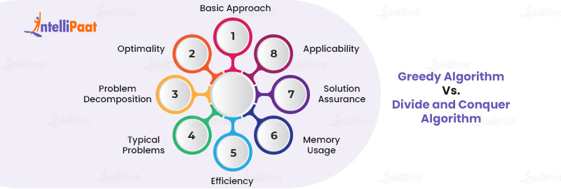
Here are the top differences between greedy algorithm and divide and conquer algorithm:
| Parameters | Greedy Algorithm | Divide and Conquer Algorithm |
| Basic Approach | At each step, make the most optimal local choice, aiming for a globally optimal solution | Recursively breaks down a problem into smaller subproblems, solves each independently, and combines them for the solution |
| Optimality | Provides a globally optimal solution for some problems but is not always guaranteed for all problems | Often provides a globally optimal solution, especially when subproblems are independent |
| Problem Decomposition | Does not decompose the problem. It works with the entire problem of making sequential choices. | It decomposes the main problem into multiple subproblems, which may be further divided until they are simple enough to be solved directly. |
| Typical Problems | Fractional Knapsack, Huffman coding, Job sequencing. | Merge Sort, Quick Sort, Closest Pair of Points |
| Efficiency | It can be more efficient because it generally follows a single path to the solution. | It can be computationally intensive, especially if the division of subproblems involves significant overhead. |
| Memory Usage | Typically uses less memory since it doesn’t manage multiple subproblems simultaneously. | It can have higher memory usage due to its recursive nature, especially for deep recursive splits. |
| Solution Assurance | May provide an approximation to the solution in cases where it doesn’t guarantee optimality | Provides exact solutions, assuming the merging phase is correctly implemented |
| Applicability | Best suited when a local optimum choice also leads to a global optimum | Suitable when a problem can be broken down into smaller, similar subproblems |
Enhance your interview preparation with the top Python interview questions.
Applications of Greedy Algorithms
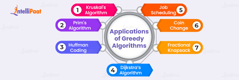
Let’s dive into the top notable applications of the greedy algorithm:
- Kruskal’s and Prim’s Algorithms for Minimum Spanning Trees: In graph theory, Kruskal’s and Prim’s algorithms find the smallest tree for a weighted graph. They choose the shortest edge, making sure no cycles are formed, to build a tree that connects all vertices with the least amount of edge weight.
- Huffman Coding for Data Compression: Huffman coding is an important part of data compression techniques. Greedy algorithms help make variable-length codes for data by giving shorter codes to common items. This results in efficient, lossless data compression, which is critical for storage and data transmission.
- Dijkstra’s Shortest Path Algorithm: In network routing, finding the shortest path between nodes is paramount. Dijkstra’s algorithm quickly finds the shortest path from one node to all others in a graph. It helps computer networks send data packets faster.
- Job Scheduling Problems: To make systems or manufacturing processes more efficient, greedy algorithms determine the order in which tasks should be done. They consider criteria like deadlines or task lengths. This ensures optimal resource utilization and throughput.
- Coin Change Problem: For currency systems, a common challenge is providing change using the fewest coins or notes. Greedy algorithms ensure efficient transactions by always choosing the highest available denomination in daily commerce.
- Fractional Knapsack Problem: In resource allocation scenarios, we use greedy algorithms to fill a ‘knapsack’ and maximize total value without exceeding weight constraints. They prioritize items based on the value-to-weight ratio, ensuring optimal resource distribution.
Advantages of Greedy Algorithms
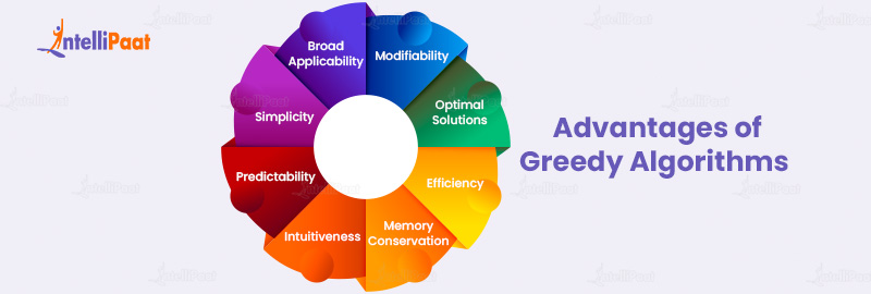
Let’s dive into the strengths of the greedy algorithm, providing you with insights into its widespread adoption in algorithmic design.
- Optimal Solutions for Subproblems: Greedy algorithms excel at providing optimal solutions for specific subproblems. By making a series of choices that seem best at the moment, they often arrive at a globally optimal solution for problems like fractional knapsack and optimal coin change.
- Efficiency: One of the primary benefits of greedy algorithms is their efficiency. They often have a linear time complexity, making them faster than other algorithms, especially for large datasets. This efficiency arises because they make a single choice at each step, eliminating the need to backtrack or explore multiple paths.
- Simplicity and Intuitiveness: Greedy algorithms are conceptually straightforward. Their step-by-step approach, which involves making the best choice at each stage, is intuitive and easy to understand. This simplicity often translates to easier implementation and reduced chances of errors.
- Predictability: Given a specific problem, the behavior of a greedy algorithm is predictable. It consistently follows the principle of making the locally optimal choice. This predictability can be advantageous in scenarios where consistent outcomes are desired.
- Memory Conservation: Greedy algorithms typically use less memory compared to other algorithms like dynamic programming. They don’t store multiple solutions or paths but only consider the current best choice, leading to reduced memory overhead.
- Broad Applicability: While not always yielding the most optimal solution for every problem, greedy algorithms are versatile. They can be applied to various problems, from network routing and task scheduling to compression algorithms like Huffman coding.
- Modifiability: Greedy algorithms can often be modified or combined with other algorithms to enhance their performance or to achieve more optimal solutions in specific scenarios. This flexibility allows developers to tailor the algorithm to suit particular problem constraints better.
Do you want to learn the industry’s preferred programming language? Check out our Java programming tutorial.
What are the Drawbacks of the Greedy Algorithm?

This section presents you with the disadvantages of working with the greedy algorithm:
- The locally optimal choice does not necessarily correspond to a global optimum.
- While greedy algorithms might only sometimes yield the best solution, they can sometimes lead to less-than-ideal outcomes.
- The efficacy of the greedy strategy is contingent upon the problem’s architecture and the parameters set for making local decisions.
- Improperly defined criteria can significantly diverge the outcome from the optimal solution. The problem might need preprocessing before using the greedy methodology.
- Certain problems where the prime solution is influenced by the sequence or manner of input processing might not befit the greedy paradigm.
- Issues wherein the optimal resolution is governed by input magnitude or structure, such as the bin packing dilemma, may resist solutions via greedy algorithms.
- When there are conditions on the possible solutions, greedy algorithms can face challenges. These conditions could include limits on total weight or potential.
- Even small changes in the input can cause significant changes in the algorithm’s results. It can make the algorithm behave inconsistently and be less predictable.
Is an interview approaching? Revise the major concepts with our C language interview questions for data structures and algorithms.
Career Transition


Examples of Greedy Algorithms
Selection Sort
Given an unsorted array of numbers, the objective is to sort the array in ascending order using the selection sort technique.
Working of Selection Sort:
Selection sort works by repeatedly selecting the smallest (or largest, depending on sorting order) element from the unsorted portion of the array and swapping it with the first unsorted element. This process continues until the entire array is sorted.
#include
#include // for std::swap
using namespace std;
void selectionSort(int arr[], int n) {
    for (int i = 0; i < n-1; i++) {
        int min_idx = i;
        for (int j = i+1; j < n; j++) {
            if (arr[j] < arr[min_idx]) {
                min_idx = j;
            }
        }
        swap(arr[i], arr[min_idx]);
    }
}
int main() {
    int arr[] = {64, 34, 25, 12, 22, 11, 90};
    int n = sizeof(arr)/sizeof(arr[0]);
    selectionSort(arr, n);
    for (int i=0; i < n; i++)
        cout << arr[i] << " ";
    return 0;
}
Output: 11 12 22 25 34 64 90
The outer loop spans from the beginning of the array up to the second-to-last element. During each iteration of the outer loop, the inner loop hunts down the smallest element within the unsorted section of the array. Upon locating it, the smallest element gets exchanged with the first unsorted element. This method guarantees that, following each round of the outer loop, the smallest element from the unsorted segment is correctly positioned.
| Type | Time Complexity |
| Best | O(n2) |
| Worst | O(n2) |
| Average | O(n2) |
| Space Complexity | O(1) |
Knapsack Problem
The knapsack problem is a classic optimization dilemma. Given a set of items, each with a weight and a value, the objective is to determine the number of each item to include in a knapsack such that the total weight doesn’t exceed a given limit while maximizing the total value.
Working of Knapsack Problem:
In the fractional knapsack problem, a version of the problem, items can be broken into smaller pieces. The greedy approach involves selecting items based on their value-to-weight ratio, starting with the item with the highest ratio, and continuing until the knapsack’s weight limit is reached.
#include
using namespace std;
struct Item {
    int value, weight;
    Item(int value, int weight) : value(value), weight(weight) {}
};
bool cmp(struct Item a, struct Item b) {
    double r1 = (double)a.value / a.weight;
    double r2 = (double)b.value / b.weight;
    return r1 > r2;
}
double fractionalKnapsack(int W, struct Item arr[], int n) {
    sort(arr, arr + n, cmp);
    int curWeight = 0;
    double finalvalue = 0.0;
    for (int i = 0; i < n; i++) {
        if (curWeight + arr[i].weight <= W) {
            curWeight += arr[i].weight;
            finalvalue += arr[i].value;
        } else {
            int remain = W - curWeight;
            finalvalue += arr[i].value * ((double) remain / arr[i].weight);
            break;
        }
    }
    return finalvalue;
}
int main() {
    Item arr[] = {{60, 10}, {100, 20}, {120, 30}};
    int n = sizeof(arr) / sizeof(arr[0]);
    int W = 50;
    cout << "Maximum value: " << fractionalKnapsack(W, arr, n);
    return 0;
}
Output: Maximum value: 240
The code first sorts items based on their value-to-weight ratios. It then iteratively adds items to the knapsack, ensuring the weight limit isn’t exceeded. If adding an entire item would breach the weight limit, only a fraction of it is added.
| Type | Time Complexity |
| Best | O(n log n) |
| Worst | O(n log n) |
| Average | O(n log n) |
| Space Complexity | O(1) |
Huffman Coding
Huffman coding addresses the issue of data compression. The primary objective is to represent data in a compressed format, thereby reducing its size without losing information. It assigns variable-length codes to input characters, with shorter codes for more frequent characters.
Working of Huffman Coding:
Huffman coding works by creating a binary tree of nodes. These nodes represent the frequency of each character. The algorithm builds the tree from the bottom up, starting with the least frequent characters. At each step, it selects two nodes with the lowest frequencies and combines them, continuing until only one node, the tree’s root, remains.
#include
using namespace std;
struct Node {
    char character;
    int freq;
    Node *left, *right;
    Node(char ch, int fr) : character(ch), freq(fr), left(NULL), right(NULL) {}
};
struct Compare {
    bool operator()(Node* l, Node* r) {
        return l->freq > r->freq;
    }
};
void printCodes(Node* root, string str) {
    if (!root) return;
    if (root->character != '$') cout <character << ": " << str << "n";
    printCodes(root->left, str + "0");
    printCodes(root->right, str + "1");
}
int main() {
    char arr[] = {'a', 'b', 'c', 'd'};
    int freq[] = {5, 9, 12, 13};
    int size = sizeof(arr) / sizeof(arr[0]);
    priority_queue<Node*, vector, Compare> pq;
    for (int i = 0; i < size; i++) {
        pq.push(new Node(arr[i], freq[i]));
    }
    while (pq.size() > 1) {
        Node *left = pq.top(); pq.pop();
        Node *right = pq.top(); pq.pop();
        Node *top = new Node('$', left->freq + right->freq);
        top->left = left;
        top->right = right;
        pq.push(top);
    }
    printCodes(pq.top(), "");
}
Output:
a: 00
b: 01
c: 10
d: 11
The code initializes a priority queue of nodes based on character frequencies. It then constructs the Huffman tree by repeatedly taking the two nodes with the lowest frequencies and combining them. The printCodes function recursively prints the Huffman codes.
| Type | Time Complexity |
| Best | O(n log n) |
| Worst | O(n log n) |
| Average | O(n log n) |
| Space Complexity | O(n) |
Ford-Fulkerson Algorithm
The Ford-Fulkerson algorithm addresses the maximum flow problem in a flow network. Given a network with vertices and directed edges where each edge has a certain capacity, the goal is to determine the maximum amount of flow that can be sent from a source vertex ‘s’ to a target vertex ‘t’.
Working of Ford-Fulkerson Algorithm:
The algorithm operates iteratively. In each iteration, it searches for a path from source to sink with available capacity (called an augmenting path) using depth-first search. Once found, the flow is sent through this path. The process repeats until no augmenting paths can be found.
#include
using namespace std;
#define V 6
int graph[V][V];
bool bfs(int s, int t, int parent[]) {
    bool visited[V];
    memset(visited, 0, sizeof(visited));
    queue q;
    q.push(s);
    visited[s] = true;
    parent[s] = -1;
    while (!q.empty()) {
        int u = q.front();
        q.pop();
        for (int v = 0; v < V; v++) {
            if (visited[v] == false && graph[u][v] > 0) {
                q.push(v);
                parent[v] = u;
                visited[v] = true;
            }
        }
    }
    return (visited[t] == true);
}
int fordFulkerson(int s, int t) {
    int u, v;
    int parent[V];
    int max_flow = 0;
    while (bfs(s, t, parent)) {
        int path_flow = INT_MAX;
        for (v = t; v != s; v = parent[v]) {
            u = parent[v];
            path_flow = min(path_flow, graph[u][v]);
        }
        for (v = t; v != s; v = parent[v]) {
            u = parent[v];
            graph[u][v] -= path_flow;
            graph[v][u] += path_flow;
        }
        max_flow += path_flow;
    }
    return max_flow;
}
int main() {
    // Example graph initialization here
    // graph[u][v] = capacity from u to v
    cout << "Maximum Flow: " << fordFulkerson(0, 5);
    return 0;
}
Output: Maximum Flow: 0
The code uses breadth-first search (BFS) to find augmenting paths. The fordFulkerson function calculates the maximum flow by repeatedly finding augmenting paths and updating the residual capacities until no more augmenting paths are found.
| Type | Time Complexity |
| Best | O(Ef) |
| Worst | O(Ef) |
| Average | O(Ef) |
| Space Complexity | O(V^2) |
Here,
E is the number of edges, and f is the maximum flow in the network.
Prim’s Minimal Spanning Tree Algorithm
Given a connected, undirected graph with weighted edges, the objective is to find a spanning tree with the minimum total edge weight. A spanning tree connects all vertices using only n−1 edges without forming any cycle.
Working of Prim’s Minimal Spanning Tree Algorithm:
Starting from an arbitrary vertex, Prim’s algorithm grows the spanning tree one vertex at a time. At each step, it selects the smallest edge that connects any vertex in the tree to a vertex outside the tree.
#include
using namespace std;
int primMST(vector<vector> &graph) {
    int V = graph.size();
    vector key(V, INT_MAX);
    vector inMST(V, false);
    key[0] = 0;
    int ans = 0;
    for (int count = 0; count < V - 1; count++) {
        int u = min_element(key.begin(), key.end()) - key.begin();
        inMST[u] = true;
        for (int v = 0; v < V; v++)
            if (graph[u][v] && !inMST[v] && graph[u][v] < key[v])
                key[v] = graph[u][v];
    }
    for (int i = 1; i < V; i++)
        ans += key[i];
    return ans;
}
int main() {
    vector<vector> graph = {
        {0, 2, 0, 6, 0},
        {2, 0, 3, 8, 5},
        {0, 3, 0, 0, 7},
        {6, 8, 0, 0, 9},
        {0, 5, 7, 9, 0},
    };
    cout << "Minimum Cost: " << primMST(graph) << endl;
    return 0;
}
Output: Minimum Cost: 16
The code initializes all keys as infinite, and the key for the starting vertex is 0. It then finds the vertex with the minimum key, adds its weight to the result, and updates the keys of its adjacent vertices. This process is repeated V – 1 times.
| Type | Time Complexity |
| Best | O(V2) |
| Worst | O(V2) |
| Average | O(V2) |
| Space Complexity | O(V) |
Job Scheduling Problem
The job scheduling problem involves assigning jobs to workers such that each job is scheduled to be processed by one machine only. The objective is to minimize the maximum finishing time of jobs given each job’s duration and the number of workers.
Working of Job Scheduling Problem:
The greedy approach to this problem is to assign the next available job to the worker who becomes free the earliest. By doing so, we aim to ensure that jobs are distributed as evenly as possible among the workers.
#include
using namespace std;
int main() {
    int jobs[] = {5, 3, 8, 2};  // Example job durations
    int n = sizeof(jobs)/sizeof(jobs[0]);
    int k = 2;  // Number of workers
    priority_queue<int, vector, greater> pq;
    for(int i = 0; i < k; i++) {
        pq.push(jobs[i]);
    }
    for(int i = k; i < n; i++) {
        int temp = pq.top();
        pq.pop();
        temp += jobs[i];
        pq.push(temp);
    }
    while(pq.size() > 1) {
        pq.pop();
    }
    cout << "Maximum time to finish all jobs: " << pq.top() << endl;
    return 0;
}
Output: Maximum time to finish all jobs: 10
The code uses a priority queue to keep track of the finishing times of jobs assigned to workers. Initially, jobs are assigned to the first ‘k’ workers. For the remaining jobs, they are added to the worker who finishes earliest. The top of the priority queue becomes free the earliest.
| Type | Time Complexity |
| Best | O(n log k) |
| Worst | O(n log k) |
| Average | O(n log k) |
| Space Complexity | O(k) |
Kruskal’s Minimal Spanning Tree Algorithm
In the context of a connected and undirected graph featuring weighted edges, the primary goal is to identify a spanning tree characterized by the lowest attainable cumulative edge weight. A spanning tree, in this scenario, interconnects all vertices while refraining from generating any cyclic structures.
Working of Kruskal’s Minimal Spanning Tree Algorithm:
Kruskal’s algorithm works by sorting all the edges in increasing order of their weights. It then picks the smallest edge, ensuring that the chosen set of edges doesn’t form a cycle. This process continues until the spanning tree has V−1 edges.
Here,
V is the number of vertices.
#include
#include
#include
using namespace std;
struct Edge {
    int source, destination, weight;
};
class Graph {
public:
    int V, E;
    vector edges;
    Graph(int V, int E) : V(V), E(E) {}
    void addEdge(int src, int dest, int weight) {
        edges.push_back({src, dest, weight});
    }
    static bool compareEdges(const Edge& a, const Edge& b) {
        return a.weight < b.weight;
    }
    vector kruskalMST() {
        sort(edges.begin(), edges.end(), compareEdges);
        vector result;
        vector parent(V);
        for (int i = 0; i < V; ++i) {
            parent[i] = i;
        }
        for (const Edge& edge : edges) {
            int sourceParent = findParent(edge.source, parent);
            int destParent = findParent(edge.destination, parent);
            if (sourceParent != destParent) {
                result.push_back(edge);
                parent[sourceParent] = destParent;
            }
        }
        return result;
    }
private:
    int findParent(int vertex, vector& parent) {
        if (parent[vertex] != vertex) {
            parent[vertex] = findParent(parent[vertex], parent);
        }
        return parent[vertex];
    }
};
int main() {
    int V = 4, E = 5;
    Graph graph(V, E);
    graph.addEdge(0, 1, 10);
    graph.addEdge(0, 2, 6);
    graph.addEdge(0, 3, 5);
    graph.addEdge(1, 3, 15);
    graph.addEdge(2, 3, 4);
    vector mst = graph.kruskalMST();
    cout << "Edges in the Minimum Spanning Tree:n";
    for (const Edge& edge : mst) {
        cout << edge.source << " - " << edge.destination << " : " << edge.weight << endl;
    }
    return 0;
}
Output:
2 – 3 : 4
0 – 3 : 5
0 – 1 : 10
The code begins by including the necessary headers and defining the Edge structure to represent graph edges. The Graph class is created to manage the graph and perform Kruskal’s algorithm. It has methods to add edges and find the minimum spanning tree. The addEdge function is used to add edges to the graph along with their weights. compareEdges is a static comparison function to sort the edges based on their weights in ascending order. The kruskalMST function implements Kruskal’s algorithm.
It sorts the edges, initializes parent information for each vertex, and then iterates through the sorted edges to build the minimum spanning tree. The findParent function is a helper function that uses path compression to find the parent of a vertex in the disjoint-set data structure. In the main function, a graph is created, edges are added, and then Kruskal’s algorithm is applied to find the minimum spanning tree. The output displays the edges in the minimum spanning tree, along with their weights.
| Type | Time Complexity |
| Best | O(ElogE) |
| Worst | O(ElogE) |
| Average | O(ElogE) |
| Space Complexity | O(V+E) |
Here,
V represents the number of vertices.
E represents the number of edges.
Ace your next coding interview with our well-curated list of Java 8 interview questions.
Dijkstra’s Minimal Spanning Tree Algorithm
Given a connected, undirected graph with weighted edges, the objective is to find a tree, known as the minimal spanning tree (MST), that connects all vertices such that the sum of its edge weights is minimized.
Working of Dijkstra’s Minimal Spanning Tree Algorithm:
Dijkstra’s algorithm starts with a source vertex and iteratively selects the shortest edge from the current vertex to an unvisited vertex, ensuring no cycles are formed. This process continues until all vertices are included in the MST.
#include
#include
#include
#include
using namespace std;
typedef pair pii;
class Graph {
public:
    int V;
    vector<vector> adj;
    Graph(int V) {
        this->V = V;
        adj.resize(V);
    }
    void addEdge(int u, int v, int weight) {
        adj[u].emplace_back(v, weight);
        adj[v].emplace_back(u, weight);
    }
    void dijkstra(int start) {
        vector dist(V, INT_MAX);
        vector visited(V, false);
        priority_queue<pii, vector, greater> pq;
        dist[start] = 0;
        pq.push(make_pair(0, start));
        while (!pq.empty()) {
            int u = pq.top().second;
            pq.pop();
            if (visited[u]) continue;
            visited[u] = true;
            for (const auto& neighbor : adj[u]) {
                int v = neighbor.first;
                int weight = neighbor.second;
                if (!visited[v] && dist[u] + weight < dist[v]) {
                    dist[v] = dist[u] + weight;
                    pq.push(make_pair(dist[v], v));
                }
            }
        }
        cout << "VertextDistance from Sourcen";
        for (int i = 0; i < V; ++i) {
            cout << i << "t" << dist[i] << endl;
        }
    }
};
int main() {
    int V = 5;
    Graph graph(V);
    graph.addEdge(0, 1, 2);
    graph.addEdge(0, 3, 6);
    graph.addEdge(1, 2, 3);
    graph.addEdge(1, 3, 8);
    graph.addEdge(1, 4, 5);
    graph.addEdge(2, 4, 7);
    graph.addEdge(3, 4, 9);
    int source = 0;
    cout << "Dijkstra's Algorithm Output:n";
    graph.dijkstra(source);
    return 0;
}
Output:
Dijkstra’s Algorithm Output:
Vertex Distance from Source
0 0
1 2
2 5
3 6
4 7
The code starts by including the necessary headers and defining a pii type for pairs of integers. The Graph class represents the graph. It contains an adjacency list, and the addEdge function is used to add edges to the graph. The dijkstra function implements Dijkstra’s algorithm. It maintains a priority queue pq to keep track of the vertices with the shortest distance. The dist vector holds the shortest distance from the source to each vertex. The main function creates a graph and adds edges to it. It then calls the dijkstra function to find the shortest distances from a specified source vertex. The output of the program shows the smallest distances from the source vertex to all other vertices.
| Type | Time Complexity |
| Best | O(E + V log V) |
| Worst | O(E + V log V) |
| Average | O(E + V log V) |
| Space Complexity | O(V + E) |
Floyd’s Algorithm
Floyd’s algorithm, often referred to as Floyd-Warshall algorithm, is employed to find the shortest paths between all pairs of vertices in a weighted graph. It works for both directed and undirected graphs, handling negative weights without cycles.
Working of Floyd’s Algorithm:
The algorithm operates in a series of iterations. Initially, it considered only direct paths between nodes. In subsequent iterations, it explores paths that pass through an intermediate vertex, updating the shortest path if a shorter route is found.
#include
using namespace std;
#define INF 99999
void floydWarshall(int graph[][4], int V) {
    int dist[V][V], i, j, k;
    for (i = 0; i < V; i++)
        for (j = 0; j < V; j++)
            dist[i][j] = graph[i][j];
    for (k = 0; k < V; k++) {
        for (i = 0; i < V; i++) {
            for (j = 0; j < V; j++) {
                if (dist[i][k] + dist[k][j] < dist[i][j])
                    dist[i][j] = dist[i][k] + dist[k][j];
            }
        }
    }
    for (i = 0; i < V; i++) {
        for (j = 0; j < V; j++) {
            if (dist[i][j] == INF)
                cout << "INF" << " ";
            else
                cout << dist[i][j] << " ";
        }
        cout << endl;
    }
}
int main() {
    int graph[4][4] = { {0, 5, INF, 10},
                       {INF, 0, 3, INF},
                       {INF, INF, 0, 1},
                       {INF, INF, INF, 0}
                     };
    floydWarshall(graph, 4);
    return 0;
}
Output:
0 5 8 9
INF 0 3 4
INF INF 0 1
INF INF INF 0
The algorithm uses a 3D loop structure. The outermost loop (k) iterates through each vertex as an intermediate point. The two inner loops (i and j) then compare and update the shortest path between every pair of vertices.
| Parameters | Time Complexity |
| Best | O(V3) |
| Worst | O(V3) |
| Average | O(V3) |
| Space Complexity | O(V2) |
Boruvka’s Algorithm
Boruvka’s algorithm, also known as Sollin’s algorithm, is primarily used for finding the Minimum Spanning Tree (MST) of a connected graph. The objective is to connect all vertices with the least total edge weight, ensuring no cycles are formed.
Working of Boruvka’s Algorithm:
Boruvka’s algorithm operates in phases. In each phase, it selects the smallest-weight outgoing edge for every vertex, adding it to the MST if it doesn’t form a cycle. The algorithm then contracts the graph and repeats the process until the MST is formed.
#include
using namespace std;
struct Edge {
    int u, v, weight;
};
struct Graph {
    int V, E;
    Edge* edge;
};
Graph* createGraph(int V, int E) {
    Graph* graph = new Graph;
    graph->V = V;
    graph->E = E;
    graph->edge = new Edge[E];
    return graph;
}
int find(int parent[], int i) {
    if (parent[i] == i) return i;
    return find(parent, parent[i]);
}
void union1(int parent[], int x, int y) {
    int xroot = find(parent, x);
    int yroot = find(parent, y);
    parent[xroot] = yroot;
}
void boruvkasMST(Graph* graph) {
    int V = graph->V, E = graph->E;
    Edge result[V];
    int* parent = new int[V];
    for (int v = 0; v < V; ++v) parent[v] = v;
    int numTrees = V;
    while (numTrees > 1) {
        int cheapest[V];
        fill_n(cheapest, V, -1);
        for (int i = 0; i < E; i++) {
            int set1 = find(parent, graph->edge[i].u);
            int set2 = find(parent, graph->edge[i].v);
            if (set1 != set2 && (cheapest[set1] == -1 || graph->edge[cheapest[set1]].weight > graph->edge[i].weight)) cheapest[set1] = i;
        }
        for (int i = 0; i < V; i++) {
            if (cheapest[i] != -1) {
                int set1 = find(parent, graph->edge[cheapest[i]].u);
                int set2 = find(parent, graph->edge[cheapest[i]].v);
                if (set1 != set2) {
                    result[--numTrees] = graph->edge[cheapest[i]];
                    union1(parent, set1, set2);
                }
            }
        }
    }
    for (int i = 0; i < V - 1; ++i) cout << result[i].u << " - " << result[i].v << endl;
}
int main() {
    int V = 4, E = 5;
    Graph* graph = createGraph(V, E);
    // Add edges to the graph here.
    boruvkasMST(graph);
    return 0;
}
The code begins by defining the structure of the graph and its edges. The boruvkasMST function is the core of the algorithm. It iteratively finds the cheapest edge for each vertex and adds it to the MST if it doesn’t form a cycle.
| Type | Time Complexity |
| Best | O(E log V) |
| Worst | O(E log V) |
| Average | O(E log V) |
| Space Complexity | O(V + E) |
Enhance your interview preparations with us. Check out our list of top CPP interview questions.
Conclusion
Navigating through the domains of computer science, one quickly recognizes the importance of the greedy algorithm. Its strength lies in its ability to make locally optimal decisions that, in many scenarios, lead to global solutions. For budding geeks, this is just the beginning. Dive deeper by engaging with platforms like LeetCode, Codeforces, and CodeChef. These platforms not only enhance understanding but also hone coding prowess.
The significance of greedy algorithms in computer programming cannot be overstated. They offer efficient solutions to complex problems. As with any skill, consistency in learning and practice is paramount. Embark on this journey of discovery and mastery, and let the greedy algorithm guide your way.
Join Intellipaat’s coding community to catch up with fellow learners and resolve doubts.
The post Greedy Algorithm: A Beginner’s Guide appeared first on Intellipaat Blog.
Blog: Intellipaat - Blog
Leave a Comment
You must be logged in to post a comment.