---

Batch Normalization: A different perspective from Quantized Inference Model

Blog: NASSCOM Official Blog

 

 

Abstract 

The benefits of Batch Normalization in training are well known for the reduction of internal covariate shift and hence optimizing the training to converge faster. This article tries to bring in a different perspective, where the quantization loss is recovered with the help of Batch Normalization layer, thus retaining the accuracy of the model. The article also gives a simplified implementation of Batch Normalization to reduce the load on edge devices which generally will have constraints on computation of neural network models.

 

Batch Normalization Theory

During the training of neural network, we have to ensure that the network learns faster. One of the ways to make it faster is by normalizing the inputs to network, along with normalization of intermittent layers of the network. This intermediate layer normalization is what is called Batch Normalization. The Advantage of Batch norm is also that it helps in minimizing internal covariate shift, as described in this paper.

The frameworks like TensorFlow, Keras and Caffe have got the same representation with different symbols attached to it. In general, the Batch Normalization can be described by following math:

 

 

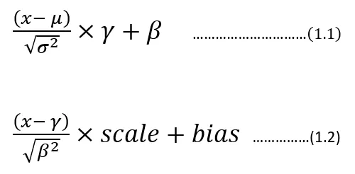
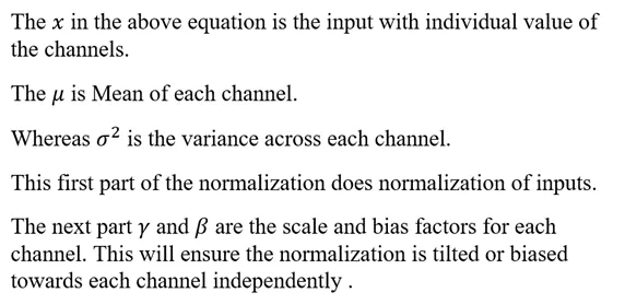
                                                                                                                                            Batch Normalization equation

 

Here the equation (1.1) is a representation of Keras/TensorFlow. whereas equation (1.2) is the representation used by Caffe framework. In this article, the equation (1.1) style is adopted for the continuation of the context.

 

Now let’s modify the equation (1.1) as below:

 

 

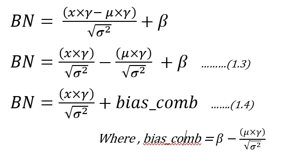
Now by observing the equation of (1.4), there remains an option for optimization in reducing number of multiplications and additions. The bias comb (read it as combined bias) factor can be offline calculated for each channel. Also the ratio of “gamma/sqrt(variance)” can be calculated offline and can be used while implementing the Batch norm equation. This equation can be used in Quantized inference model, to reduce the complexity.

Quantized Inference Model

The inference model to be deployed in edge devices, would generally integer arithmetic friendly CPUs, such as ARM Cortex-M/A series processors or FPGA devices. Now to make inference model friendly to the architecture of the edge devices, will create a simulation in Python. And then convert the inference model’s chain of inputs, weights, and outputs into fixed point format. In the fixed point format, Q for 8 bits is chosen to represent with integer.fractional format. This simulation model will help you to develop the inference model faster on the device and also will help you to evaluate the accuracy of the model.

e.g: Q2.6 represents 6 bits of fractional and 2 bits of an integer.

Now the way to represent the Q format for each layer is as follows:

1. Take the Maximum and Minimum of inputs, outputs, and each layer/weights.
2. Get the fractional bits required to represent the Dynamic range (by using Maximum/Minimum) is as below using Python function:

def get_fract_bits(tensor_float):
  # Assumption is that out of 8 bits, one bit is used as sign
  fract_dout = 7 - np.ceil(np.log2(abs(tensor_float).max()))

  fract_dout = fract_dout.astype('int8')

  return fract_dout

3. Now the integer bits are 7-fractional_bits, as one bit is reserved for sign representation.
   4. To start with perform this on input and then followed by Layer 1, 2 …, so on.
   5. Do the quantization step for weights and then for the output assuming one example of input. The assumption is made that input is normalized so that we can generalize the Q format, otherwise, this may lead to some loss in data when non-normalized different input gets fed.
   6. This will set Q format for input, weights, and outputs.

Example:
Let’s consider Resnet-50 as a model to be quantized. Let’s use Keras inbuilt Resnet-50 trained with Imagenet.

#Creating the model

def model_create():

    model = tf.compat.v1.keras.applications.resnet50.ResNet50(

    include_top=True,

    weights='imagenet',

    input_tensor=None,

    input_shape=None,

pooling=None,

    classes=1000)

    return model

 

Let’s prepare input for resnet-50. The below image is taken from ImageNet dataset.

 

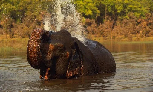
def prepare_input():

      img = image.load_img(

            "D:Elephant_water.jpg",

            target_size=(224,224)

            )

      x_test = image.img_to_array(img)

      x_test = np.expand_dims(x_test,axis=0)

      x = preprocess_input(x_test) # from tensorflow.compat.v1.keras.applications.resnet50 import preprocess_input, decode_predictions

      return x

Now Lets call the above two functions and find out the Q format for input.

      model = model_create()

      x     = prepare_input()

If you observe the input ‘x’, its dynamic range is between -123.68 to 131.32. This makes it hard for fitting in 8 bits, as we only have 7 bits to represent these numbers, considering one sign bit. Hence the Q Format for this input would become, Q8.0, where 7 bits are input numbers and 1 sign bit. Hence it clips the data between -128 to +127 (-2⁷ to 2⁷ -1). so we would be loosing some data in this input quantization conversion (most obvious being 131.32 is clipped to 127), whose loss can be seen by Signal to Quantize Noise Ratio , which will be described soon below.

If you follow the same method for each weight and outputs of the layers, we will have some Q format which we can fix to simulate the quantization.

       # Lets get first layer properties

       (padding, _) = model.layers[1].padding

       # lets get second layer properties

       wts = model.layers[2].get_weights()

       strides = model.layers[2].strides

       W=wts[0]

       b=wts[1]

 

       hparameters =dict(

                    pad=padding[0],

                    stride=strides[0]

                   )

         # Lets Quantize the weights .

         quant_bits = 8 # This will be our data path.

         wts_qn,wts_bits_fract = Quantize(W,quant_bits) # Both weights and biases will be quantized with wts_bits_fract.

         # lets quantize Bias also at wts_bits_fract

         b_qn = (np.round(b *(2<<wts_bits_fract))).astype('int8')

         names_model,names_pair = getnames_layers(model)

         layers_op = get_each_layers(model,x,names_model)

         quant_bits = 8

         print("Running conv2D")

         # Lets extract the first layer output from convolution block.

         Z_fl = layers_op[2] # This Number is first convolution.

         # Find out the maximum bits required for final convolved value.

         fract_dout = get_fract_bits(Z_fl)

         fractional_bits = [0,wts_bits_fract,fract_dout]

         # Quantized convolution here.
         Z, cache_conv = conv_forward(

                         x.astype('int8'),

                         wts_qn,

                         b_qn[np.newaxis,np.newaxis,np.newaxis,...],

                         hparameters,

                         fractional_bits)

Now if you observe the above snippet of code, the convolution operation will take input, weights, and output with its fractional bits defined.
i.e: fractional_bits=[0,7,-3]
where 1st element represents 0 bits for fractional representation of input (Q8.0)
2nd element represents 7 bits for fractional representation of weights (Q1.7).
3rd element represents -3 bits for the fractional representation of outputs (Q8.0, but need additional 3 bits for integer representation as the range is beyond 8-bit representation).

This will have to repeat for each layer to get the Q format.

Now the quantization familiarity is established, we can move to the impact of this quantization on SQNR and hence accuracy.

Signal to Quantization Noise Ratio

As we have reduced the dynamic range from floating point representation to fixed point representation by using Q format, we have discretized the values to nearest possible integer representation. This introduces the quantization noise, which can be quantified mathematically by Signal to Quantization noise ratio.(refer: https://en.wikipedia.org/wiki/Signal-to-quantization-noise_ratio)

As shown in the above equation, we will measure the ratio of signal power to noise power. This representation applied on log scale converts to dB (10log10SQNR). Here signal is floating point input which we are quantizing to nearest integer and noise is Quantization noise.
example: The elephant example of input has maximum value of 131.32, but we are representing this to nearest integer possible, which is 127. Hence it makes Quantization noise = 131.32–127 = 4.32.
So SQNR = 131.32² /4.32² = 924.04, which is 29.66 db, indicating that we have only attained close to 30dB as compared to 48dB (6*no_of_bits) possibility.

This reflection of SQNR on accuracy can be established for each individual network depending on structure. But indirectly we can say better the SQNR the higher is the accuracy.

Convolution in Quantized environments:

The convolution operation in CNN is well known, where we multiply the kernel with input and accumulate to get the results. In this process we have to remember that we are operating with 8 bits as inputs , hence the result of multiplication need at least 16 bits and then accumulating it in 32 bits accumulator, which would help to maintain the precision of the result. Then result is rounded or truncated to 8 bits to carry 8 bit width of data.

def conv_single_step_quantized(a_slice_prev, W, b,ip_fract,wt_fract,fract_dout):

 """

 Apply one filter defined by parameters W on a single slice (a_slice_prev) of the output     activation

 of the previous layer.

 Arguments:

 a_slice_prev -- slice of input data of shape (f, f, n_C_prev)

 W -- Weight parameters contained in a window - matrix of shape (f, f, n_C_prev)

 b -- Bias parameters contained in a window - matrix of shape (1, 1, 1)

Returns:

 Z -- a scalar value, result of convolving the sliding window (W, b) on a slice x of the     input data

"""

       # Element-wise product between a_slice and W. Do not add the bias yet.

       s = np.multiply(a_slice_prev.astype('int16'),W) # Let result be held in 16 bit

       # Sum over all entries of the volume s.

       Z = np.sum(s.astype('int32')) # Final result be stored in int32.

       # The Result of 32 bit is to be trucated to 8 bit to restore the data path.

       # Add bias b to Z. Cast b to a float() so that Z results in a scalar value.

       # Bring bias to 32 bits to add to Z.

       Z = Z + (b << ip_fract).astype('int32')

       # Lets find out how many integer bits are taken during addition.

       # You can do this by taking leading no of bits in C/Assembly/FPGA programming

       # Here lets simulate

       Z = Z >> (ip_fract+wt_fract - fract_dout)

       if(Z > 127):

             Z = 127

       elif(Z < -128):

             Z = -128

       else:

            Z = Z.astype('int8')

       return Z

The above code is inspired from AndrewNg’s deep learning specialization course, where convolution from scratch is taught. Then modified the same to fit for Quantization.

Batch Norm in Quantized environment

As shown in Equation 1.4, we have modified representation to reduce complexity and perform the Batch normalization.The code below shows the same implementation.

def calculate_bn(x,bn_param,Bn_fract_dout):

        x_ip = x[0]
        x_fract_bits = x[1]

       bn_param_gamma_s = bn_param[0][0]

       bn_param_fract_bits = bn_param[0][1]

       op = x_ip*bn_param_gamma_s.astype(np.int16) # x*gamma_s

       # This output will have x_fract_bits + bn_param_fract_bits

       fract_bits =x_fract_bits + bn_param_fract_bits

       bn_param_bias = bn_param[1][0]

       bn_param_fract_bits = bn_param[1][1]

       bias = bn_param_bias.astype(np.int16)

       # lets adjust bias to fract bits

       bias = bias << (fract_bits - bn_param_fract_bits)

       op = op + bias # + bias

       # Convert this op back to 8 bits, with Bn_fract_dout as fractional bits

       op = op >> (fract_bits - Bn_fract_dout)

       BN_op = op.astype(np.int8)

       return BN_op

Now with these pieces in place for the Quantization inference model, we can see now the Batch norm impact on quantization.

Results

The Resnet-50 trained with ImageNet is used for python simulation to quantize the inference model. From the above sections, we bind the pieces together to only analyze the first convolution followed by Batch Norm layer.

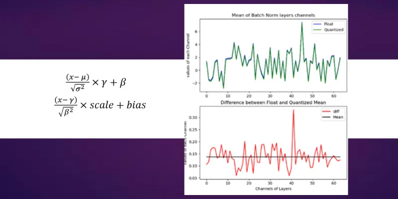
The convolution operation is the heaviest of the network in terms of complexity and also in maintaining accuracy of the model. So let’s look at the Convolution data after we quantized it to 8 bits. The below figure on the left-hand side represents the convolution output of 64 channels (or filters applied) output whose mean value is taken for comparison. The Blue color is float reference and the green color is Quantized implementation. The difference plot (Left-Hand side) gives an indication of how much variation exists between float and quantized one. The line drawn in that Difference figure is mean, whose value is around 4. which means we are getting on an average difference between float and Quantized values close to a value of 4.

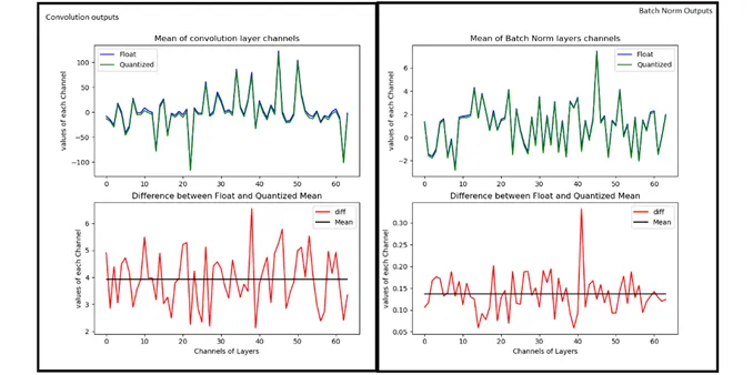
                                                                                                                                    Convolution and Batch Norm Outputs

 

Now let’s look at Right-Hand side figure, which is Batch Normalization section. As you can see the Green and blue curves are so close by and their differences range is shrunk to less than 0.5 range. The Mean line is around 0.135, which used to be around 4 in the case of convolution. This indicates we are reducing our differences between float and quantized implementation from mean of 4 to 0.135 (almost close to 0).

 

Now let’s look at the SQNR plot to appreciate the Batch Norm impact.

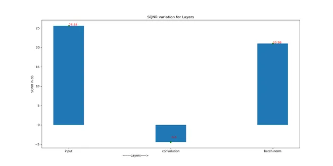
                                                                                                                      Signal to Quantization Noise Ratio for sequence of layers

 

Just in case values are not visible, we have following SQNR numbers
Input SQNR : 25.58 dB (The Input going in to Model)
Convolution SQNR : -4.4dB (The output of 1st convolution )
Batch-Norm SQNR : 20.98 dB (The Batch Normalization output)

As you can see the input SQNR is about 25.58dB , which gets reduced to -4.4 dB indicating huge loss here, because of limitation in representation beyond 8 bits. But the Hope is not lost, as Batch normalization helps to recover back your SQNR to 20.98 dB bringing it close to input SQNR.

Conclusion

1. Batch Normalization helps to correct the Mean, thus regularizing the quantization variation across the channels.
2. Batch Normalization recovers the SQNR. As seen from above demonstration, we see a recovery of SQNR as compared to convolution layer.
3. If the quantized inference model on edge is desirable, then consider including Batch Normalization as it acts as recovery of quantization loss and also helps in maintaining the accuracy, along with training benefits of faster convergence.
4. Batch Normalization complexity can be reduced by using (1.4) so that many parameters can be computed offline to reduce load on the edge device.

References

• https://medium.com/r/?url=https%3A%2F%2Farxiv.org%2Fpdf%2F1502.03167.pdf
• https://www.coursera.org/specializations/deep-learning
• https://en.wikipedia.org/wiki/Signal-to-quantization-noise_ratio

 

The post Batch Normalization: A different perspective from Quantized Inference Model appeared first on NASSCOM Community |The Official Community of Indian IT Industry.