
Why Does DMN Have BKMs?
Blog: Method & Style (Bruce Silver)
Newcomers to DMN may wonder, What is the point of Business Knowledge Models (BKMs), those funny-looking boxes with clipped corners in the DRD? When I was first introduced to DMN, struggling to understand the DMN 1.0 spec, I wondered the same thing. The spec was (and remains) largely impenetrable to decision modelers, except for the example model in Chapter 11. That example has a BKM attached to every decision in the DRD, but for no obvious reason. The BKMs just seem to add clutter and complexity to the decision model. And, to be honest, a number of so-called DMN tools don’t support BKMs at all! What’s going on here?
It turns out there are a number of excellent reasons to use BKMs. After reading this post, maybe you’ll use them more in your own decision models.
Let’s start with a simple decision model. This typically would be just a fragment of a larger decision, but let’s just focus on this small part, calculating the monthly loan payment for a home mortgage. Here is the DRD:
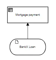
The input data BankX Loan has three components:
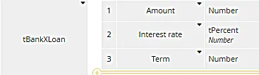
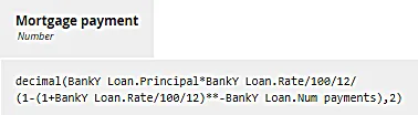
The decision Mortgage payment simply calculates the monthly payment based on those component values using the well-known amortization formula:
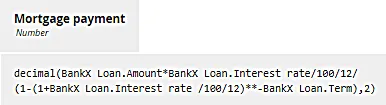
Wow, that’s a mouthful! Yes, the formula is “well-known” in the sense that it’s used all the time in mortgage lending, but do we expect a decision modeler to be able to enter it from memory, or even type it in correctly? Maybe not. Let’s say this decision is used by a mortgage broker who is dealing with a number of lenders. BankY’s data looks like this:
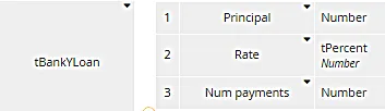
It’s the same information BankX uses, but BankY uses different names: Principal instead of Amount, Rate instead of Interest rate, etc. The amortization formula for BankY looks different because it has to use the new names:
This simple example points out several problems where BKMs can offer some help. First, the decision modeler may know that a formula exists to calculate the loan payment given the loan amount, interest rate, and term, but has no idea what it is. Second, even knowing the formula, the FEEL expression involves the specific names of the loan components, which differ from lender to lender. And third, you want this calculation to work exactly the same way with every lender. Deep down, the formula is the same, even though the names of the variables change from one lender to the next. You’d prefer to be able to reuse the formula in any decision logic, no matter what the input data elements in the DRD are called.
Fundamentally this is what a BKM does. It expresses decision logic as a parameterized function. The names of the parameters – the inputs to the logic – are defined by the BKM itself, not by the particular decision model that uses it. The decision model that uses it simply “invokes” – that is, calls – the BKM, passing values to each of its parameters and receiving the BKM result back in return. That solves all three problems above.
- The modeler who knows what the decision requirement is but does not know how to implement it may incorporate that implementation, created by someone else, a subject matter expert, in the decision. The modeler does not need to know how to develop the decision logic, or even how it works. He or she simply needs to know how to invoke it, and this – as you’ll see – is very easy. That is part of what DMN’s originators had in mind when they included BKMs in the standard. More on that later.
- Second, the FEEL expression in the BKM is independent of the variable names used in each calling model. That allows the formula to be shorter and easier to understand.
- And third, the BKM by definition works the same in every decision model that uses it.
Here are the DRDs for BankX and BankY using BKMs:
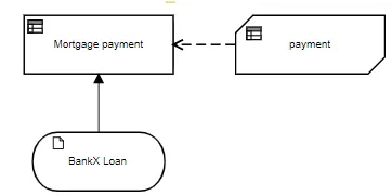
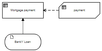
They look the same, and the BKM payment is exactly the same in both:
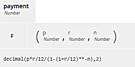
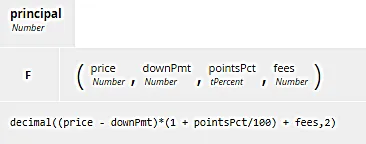
What you see here is the boxed expression for a BKM. The code F means FEEL, the default. A BKM could also invoke external logic, specifically Java (code J) or PMML (code P). To the right of that are the three parameters. Here they are p, the principal or loan amount; r, the loan rate expressed as a decimal not a percent; and n, the number of months in the loan term. We could name them whatever we want. They are used only by the BKM’s internal logic. The amortization formula, expressed in terms of p, r, and n, is shorter than we saw previously. The decimal() function wrapping the arithmetic expression simply rounds the result to two decimal places. This formula is used for both BankX and BankY.
What is different in the two DRDs above is the invocation of the BKM performed by the decision Mortgage payment. The invoking decision simply has to map its inputs – here the components of either BankX Loan or BankY Loan, to the BKM parameters p, r, and n. There are two different ways to do this, and both are easy.
The first way, called literal invocation, doesn’t refer to the parameter names at all, just their order in the BKM definition. As you see above, p is the first parameter, r the second, and n the third. So for BankX’s Mortgage payment we have this:
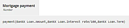
Literal invocation means a FEEL literal expression with the name of the BKM followed by its arguments – values of its parameters, in the correct order – in parentheses. So here the first argument, BankX Loan.Amount, is mapped to parameter p; the second argument, BankX Loan.Interest rate/100, is mapped to parameter r; and the third argument, BankX Loan.Term, is mapped to parameter n. We had to divide by 100 in the second argument in order to convert the rate expressed as percent to a decimal value. If we used literal invocation for BankY, the arguments would reference the variable names used by that lender.
But for BankY, we won’t do it that way. Instead of literal invocation, here we illustrate boxed invocation, a standard tabular format for invoking BKMs. It’s a two-column table with the parameter names in the first column and the mapping expression in the second column. It looks like this:
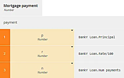
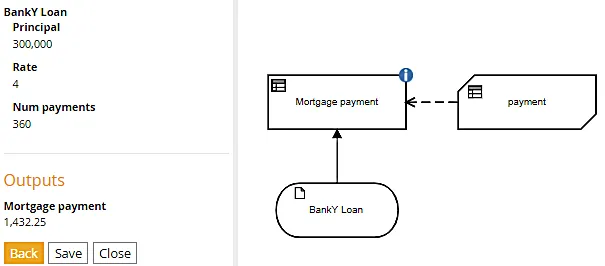
The name of the invoked BKM, payment, is at the top. Below that is the two-column table, the BKM parameter names on the left, and the mapping expression for each on the right. The boxed invocation is maybe easier for beginners to understand, but both forms of the invocation work the same way and give the same result on execution. For a 30 year loan of $300,000 at an annual rate of 4%, the payment is $1432.25.
Now if you’ve ever shopped for a home loan, you know it’s a little more complicated than this. In addition to the annual loan rate, lenders often charge points – a percentage of the requested loan amount – and possible a fixed fee. In most cases, these extra amounts are amortized along with the original requested amount, increasing the loan amount. So in reality, comparing the monthly payment between lenders requires taking this into account as well.
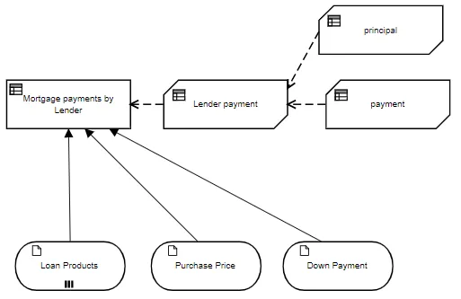
So here is a more complex DRD that involves multiple BKMs. The decision Mortgage payments by Lender returns a table of monthly payments by lender by invoking BKM Lender payment, which in turn invokes two BKMs, principal and payment. The connection of the called element to the calling element is indicated in the diagram by the dashed arrow, called a knowledge requirement. Here input data Loan Products is a table of lender offerings, specifying the interest rate, points, and fees:
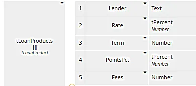
Its datatype tLoanProducts is a collection (list) of the row type tLoanProduct, with the five components shown here. Here we see another use of BKMs, iteration over a list. The decision Mortgage payments by lender is also a table, one row per row of Loan Products, simply showing the lender name and the calculated monthly payment given values for the Purchase price, Down payment, and Loan Product details. We need to create this table one row at a time using iteration:
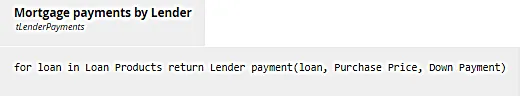
Iteration uses the FEEL syntax
for [range variable] in [list variable] return [expression of range variable]
where the range variable is simply a name meaning one item in the list – here one row of Loan Products, and the expression is a literal invocation of the BKM Lender payment. Note that the first argument is the range variable loan, again meaning a row of Loan Products, a structure with the five components shown above.
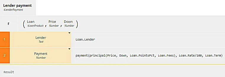
Here you see the definition of the BKM Lender payment. The parameters are Loan, Price and Down. Note the datatype of each parameter must match the type of the arguments passed in the invocation. This BKM returns a row of Mortgage payments by lender, which has two components, Lender (the lender name) and Payment. The way to create such a structure is with a context, another boxed expression type, having a row (context entry) for each component of the output, its name in the first column and value expression in the second column, and an empty final result box (the bottom row, labeled Result). The component Lender is taken from Loan, which is a row of Loan Products. The component Payment has a more complicated value expression, illustrating what you can do with BKM invocation. It invokes the BKM payment, and for the first argument invokes the BKM principal, which calculates the loan amount. In other words, Mortgage payments by lender invokes the BKM Lender payment, which in turn invokes the BKM payment and – as an argument of payment – the BKM principal.
If you don’t like the complicated nested literal expression above, you might find nesting boxed invocations more understandable if less compact:
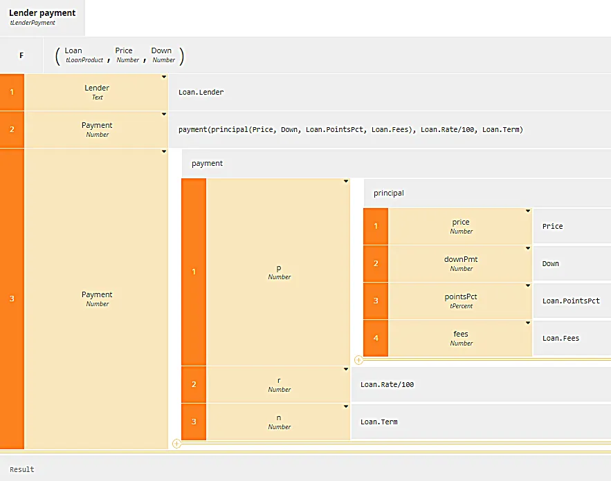
The BKM principal calculates the total loan amount from the price, down payment, lender points and fees, and this is used in turn to calculate the monthly loan payment for that lender.
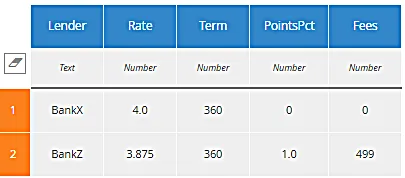
It can make your head spin, but when working with tables such use of BKMs is not uncommon. Let’s try it out. Here is a short table for BankX, which offers a 4% loan with no points or fees, and BankZ, which offers a 3.875% loan with 1% points and $499 fees. Which has the lower monthly payment? It’s not obvious from inspection.
When we run the model with Purchase Price $375,000, Down Payment $75,000, we get this:
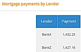
BankZ has a lower monthly payment, but only slightly.
When dealing with lists and tables, BKMs are indispensable. They let you work on each item in the list or row in the table at a time, and iterate the result.
Many of these BKM benefits arise from its nature as reusable decision logic. In fact, it is common to save BKMs in a library and simply import them into any decision model that needs that bit of logic. Nevertheless, the creator of the BKM idea has always insisted that his motivation for BKMs was never reuse, but methodology. This goes to a deeper issue, a somewhat divisive one within the decision management community. I’ll address it briefly here and possibly return to it in a future post.
BKMs originated in a FICO methodology called Decision Requirements Analysis. The idea is that a complex decision model, as expressed in the DRD, requires”knowledge” not available to the DRD modeler but instead distributed across a variety of subject matter experts in the organization. Thus the DRD modeler, capturing the end-to-end view, defines only the decision requirements, the names of each decision node, its datatype, and the names and types of its inputs. The actual decision logic generating the output from the inputs is implicitly created by someone else, a subject matter expert in that specific part of the logic. BKMs allow the DRD modeler and BKM authors to work independently and glue their contributions together using invocation.
I think this is why all the decisions in the spec Chapter 11 example have attached BKMs. The example is a little misleading in that the BKM logic is not especially reusable or too difficult for the modeler to figure out for himself. It simply illustrates the structure implied by that methodology.
Hmmm… OK. But why not simply incorporate the decision logic directly in the decision node? That’s what the FEEL language, designed for business users, was expressly intended to do! The unspoken part of the above methodology is that these subject matter experts are not using FEEL. They are using a programming language like Java or a proprietary rule engine language. Encapsulating that programming in a BKM allows FEEL – the language of the DRD – to be mapped to the programming language. This separation between decision requirements created by business and logic implementation created by programmers is what DMN supposedly was trying to avoid. The key idea – the reason why FEEL has names with spaces and other “business-friendly” attributes – was always that business wants to “own” its decision logic. That means being able to create and test it themselves. The methodological rationale for BKMs at least gets you halfway there. While implementation may be delegated to programmers, encapsulating it in BKMs at least allows business to test the end-to-end DRD logic themselves.
That is in contrast to some tools that create DMN-like DRDs but simply link decision nodes directly to a proprietary implementation. Those are the tools that claim to be DMN but don’t support BKMs at all. To me, that’s using DMN simply as a RFP checkoff item, not as a true standard. In those tools, business is confined to its traditional role of creating requirements handed off to programmers. I’m not sure how that is better than doing the whole thing in the proprietary business rule environment.
Whether decision logic implementation is done in FEEL by non-programmers or delegated to programmers in some other language, BKMs in the end allow business to own the end-to-end decision logic and test for itself that it is valid and complete.
The post Why Does DMN Have BKMs? appeared first on Method and Style.