Read Blog Post

Read Blog Post

Contributed on October 16, 2011

2

335

Inside Nitro: The Timeframe Filter

With Nitro 3.0 we introduced log filters. Filtering is as essential tool to clean your data and to drill down into specific aspects of your process. Last time, I explained how the Endpoint filter works, and when and why you need it.

Today, I want to show you the power of the Timeframe filter. Like most filters, the timeframe filter can be used both for data cleaning and for focusing your analysis. I’ll start with a data cleaning example.

1. Remove cases with timestamps in the future

More than once I have encountered data sets with erroneous timestamps that lie outside the boundaries of the analyzed data.

This could happen because the timestamps for some of the activities in the process are recorded manually. In comparison to the automatically recorded timestamps, these errors are relatively rare exceptions. However, because timestamps are important for the order of activities and the throughput time analysis, we want to remove them.

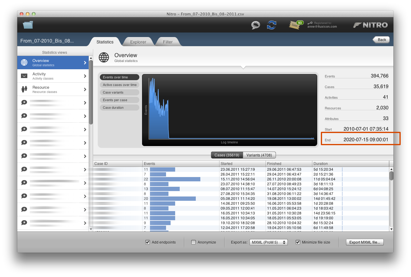
The data set contains timestamps of the year 2020 (click on the image to see a larger version).

When we open the Filter tab for this data set, Nitro recommends to use the Timeframe filter. We can add the Timeframe filter by clicking the button ‘Add filter’, or alternatively select the filter directly in the top-left corner as explained the last time.

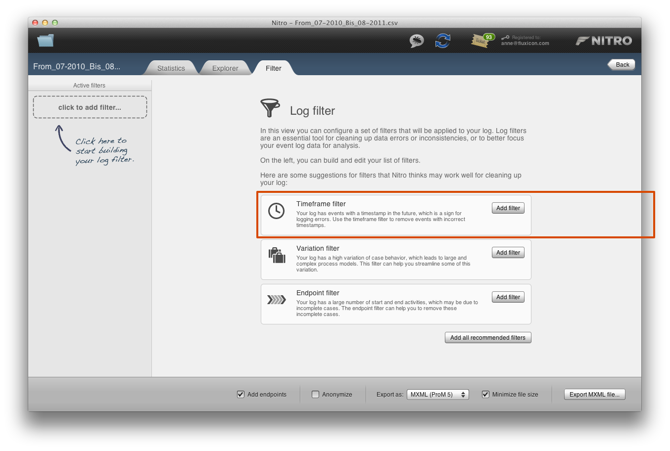
Nitro is smart enough to detect that some timestamps lie in the future and recommends to use the Timeframe filter.

Initially, the start and end time are set to the earliest and latest timestamp in the overall log — so the complete log is covered. The timeframe can then be changed interactively by simply moving the slider at the left or right end of the timeframe, or by providing the desired start and end date and time directly. In our example, we keep the start date of the log but change the end time to today’s date, because we we want to get rid of all future timestamps.

The resulting time frame area of the current selection is highlighted in blue on top of a visualization of the number of active cases over time. This visualization helps you to see how many cases are affected: A low value on the y-axis (a valley or low-land) means that only few cases are running at that point in time. A high-value on the y-axis (a mountain or high-land) means that many cases are running.

After the filter is applied, only those cases that are started and completed within the selected timeframe are kept.

It’s really easy to adjust the timeframe by simply moving the slider. We set the end date around the current date to get rid of the future timestamps.

The filtering result for the example data set can be seen in the screenshot below: There are four cases less than in the unfiltered log (35,615 instead of 35,619). These were process instances that had events with timestamps in the future.

The latest timestamp is now 1 September 2011.

Usage modes of the Timeframe filter

So far, I have used the standard mode of the Timeframe filter, where only cases that completely lie within the selected timeframe are kept. There are other usage modes, which:

• keep cases that are starting in the selected timeframe,
• keep cases that are completed within the selected timeframe,
• keep cases that are either started or completed (intersecting) within the selected timeframe,
• or trim cases to the selected timeframe.

Here is an overview of all the available Timeframe filter settings:

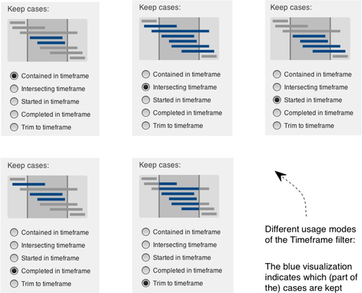
When you change the usage mode, the blue visualizations adapt to help you understand the effect of the mode you are currently using.

In fact, instead of removing the four cases with the timestamps from 2020, I decided to manually correct and include them in the analysis.

To find these erroneous timestamps, I had to use the timeframe filter not to remove but to detect cases with timestamps in the future. So, I used the ‘Intersect’ mode in combination with the timeframe ranging from the current date (today) up to the end of the log. This way, only the four cases that had outlier timestamps in the future remained, and I could write down their caseIDs to fix the dates in the original data set¹.

2. Compare a process for two different months

Beyond just correcting errors in the logging, the timeframe filter is perfect for slicing up the data according to time criteria.

For example, let’s say that you need to compare the throughput times for February and April in another process. You know that in March a process change has been introduced that, theoretically, should push all cases running longer than 5 days into a special queue. The cases in this queue then get priority treatment by a separate team. You want to know whether the change had the desired effect of limiting the process throughput time to a maximum of 10 days.

To do this comparison, you need to isolate process instances that were started in February (before the change) and in April (after the change). First, the February cases are selected using the timeframe filter:

1. Set 1 February (00:00:00) as the start date.

2. Set 1 March (00:00:00) as the end date.

3. Change the Timeframe filter settings to ‘Started in timeframe’

4. Click ‘Start filtering…’

Select all cases that were started in February.

After applying the filter, you have a list of all process instances that were started in February in the Statistics overview of Nitro. This table also contains the individual throughput times. Simply right-click that table to export the table data as a CSV file. This works for all tables in Nitro.

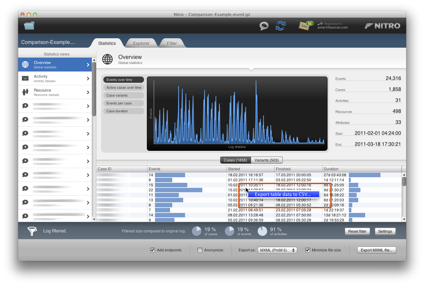
Right-click the table with the throughput times and export it as a CSV file.

When you open the exported CSV file in Excel, you will see that the throughput times (Duration) are in milliseconds. This gives you the full flexibility to display the data in whatever time unit you want. Simply change the time unit by adding a second column that recalculates your throughput times, for example, to days.

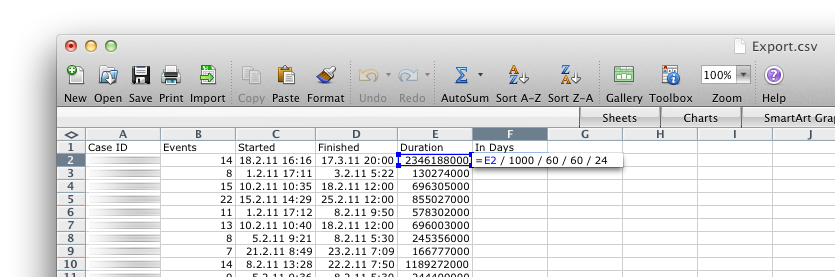
Adjust the time unit for your throughput times in Excel.

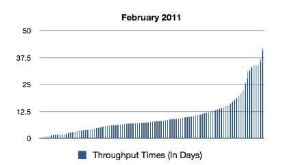
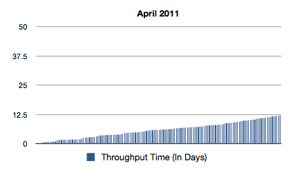
After you have repeated the same procedure for your April data, the throughput times for the two months can be displayed in a chart, for example, using Excel. From the result, one can see that the process change had an intense effect: Before the change, some cases were running up to around 40 days — After the change, none of them runs longer than 13 days.

Of course, you can also compare the process flows, statistics, conformance, or other process mining results for these two months. Furthermore, multiple Timeframe filters can be combined to refine the results even further: Think of filtering all cases that were started in week 1 and completed in week 3 of a certain month, for example.

I find the Timeframe filter essential for my own work. And I just love to use it because it is so visual and quickly does what I want. If you haven’t tried it yet, go download the free demo version of Nitro here, and play with the sample data set that comes with the download.