
Fraud Analytics for Open Banking: Multi-Layered Self-Calibrating Models
Blog: Enterprise Decision Management Blog

In my previous post, I described how fraud analytics for open banking work. Following an introduction to behavioral analytics, this post focuses on how the data refined through behavioral profiles are combined in an unsupervised machine learning model to produce a score indicative of fraud or non-fraud.
Rationale for Utilising Unsupervised Models
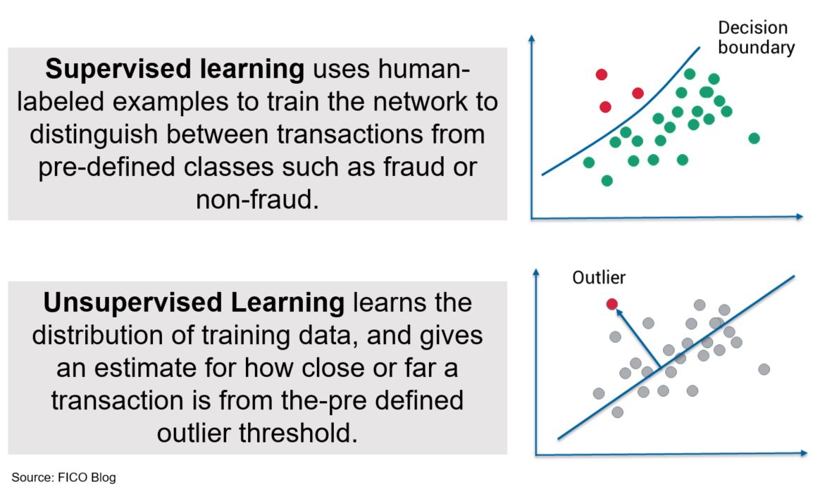
Regarding fraud analytics for open banking, where historical data is not yet available and the evolution of open banking in terms of adoption is still unclear, unsupervised machine learning can be a strong weapon for fighting financial crime events. Without adequate labelled historical data, supervised machine learning models such as neural networks can’t be built. Therefore, unsupervised machine learning models provide a valuable alternative.
FICO’s unsupervised machine learning technology is called Multi-Layered Self-Calibrating (MLSC) models and was developed and patented by FICO to determine how unusual the transaction is, based on key feature detectors often derived based on expert knowledge to determine risky behaviors in production.
Figure 1. Supervised vs. Unsupervised Learning in FICO Falcon Platform
Introduction to Self-Calibration and Quantiles
Generally, self-calibration is defined as a model’s ability to adjust to the changes in the distributions of predictive variables in order to, for example, accommodate evolving payment transfer patterns and adapt to economic shifts.
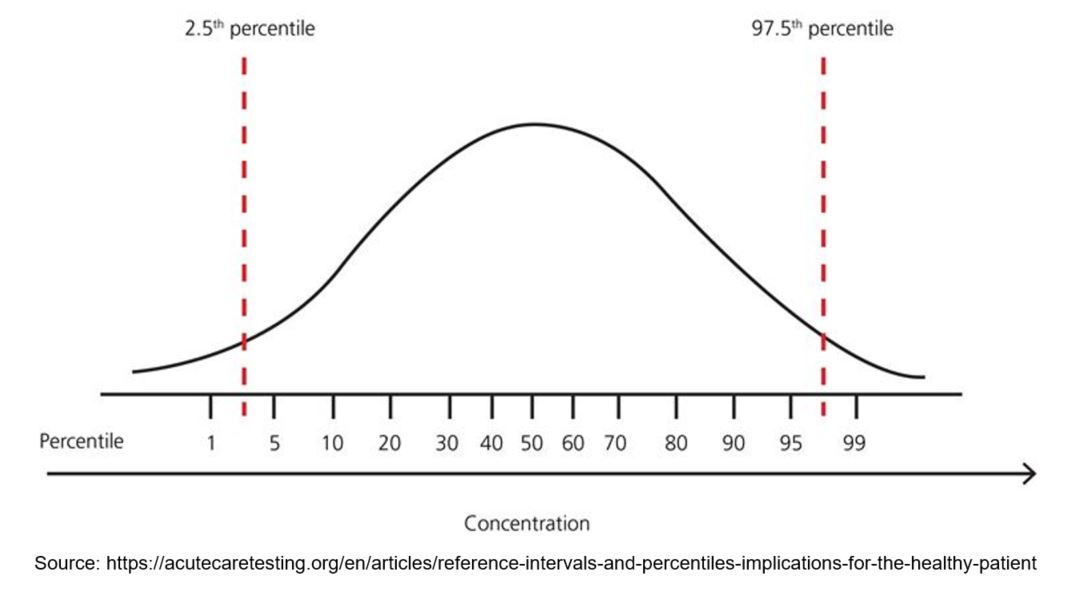
A quantile is where a data sample is divided into equal-sized, adjacent subgroups. For example, the median is a quantile that is placed in a probability distribution so that one half of the data is below the median and the other half is above the median. Percentiles are quantiles that split a distribution into 100 equal parts (Figure 2).
Figure 2. Percentiles in a Distribution
MLSC Models
MLSC models use machine learning and statistical techniques to dynamically scale variables, estimate variable value distributions and determine the outliers in key feature detectors, and then compute latent features that are in general more predictive than the inputs on their own.
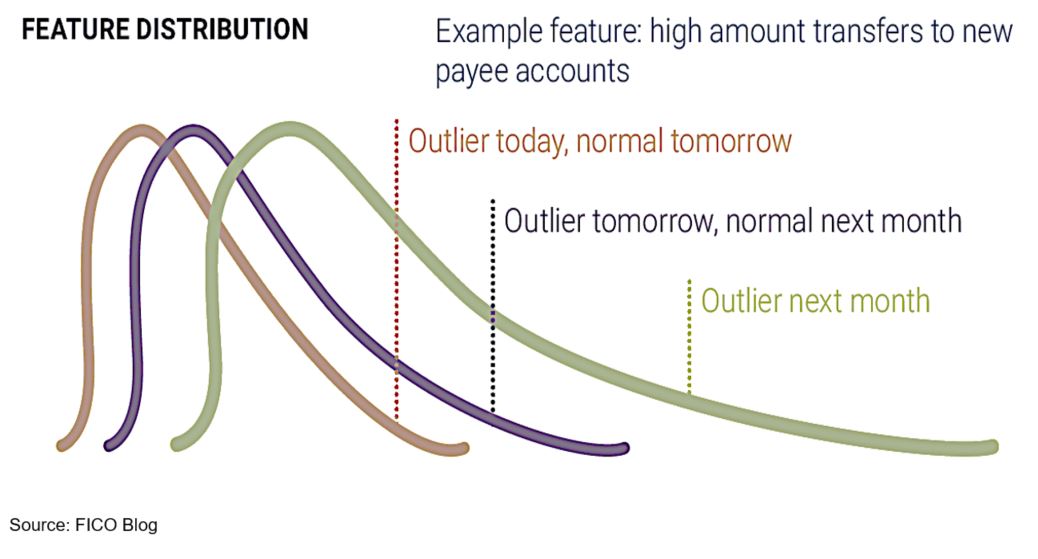
For example, Figure 3 shows the distribution of high amount transfers to new payee accounts, and the distribution relative to accounts within the same peer group. The distribution of this feature is expected to change over time, due to the dynamic nature of the open banking environment. In other words, percentile thresholds for being an outlier can be different on a day-to-day basis; what is an outlier today may be normal tomorrow. Therefore, for a model to be robust, it must re-calculate the values of percentile thresholds “on the fly”, in a production environment.
Regardless of a distribution type (normal vs. non-normal), percentiles can be used as outlier thresholds.
Figure 3. Changes in the Distribution of High Amount Transfers to New Payee Accounts
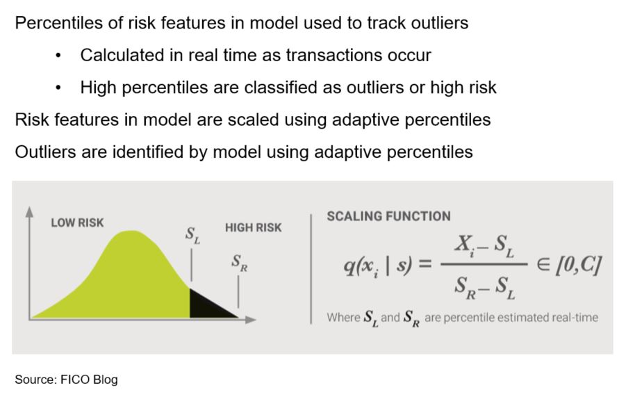
In MLSC models, as previously mentioned, abnormal behavior is measured based on quantiles. The normalizing parameters used to scale inputs are percentile estimates that are derived and updated each time a new transaction comes into the FICO Falcon Platform (Figure 4). MLSC models learn from transactions in production, adjusting as behavior patterns change over time.
Figure 4. Adaptive Outlier Detection in MLSC Models
It is important to recognize that MLSC models resemble neural networks because they merge the properties of neural networks with adaptive outlier detection (Figure 5).
Figure 5. Traditional Neural Network Versus MLSC Model
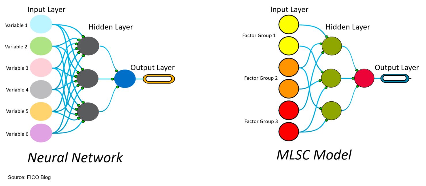
In a neural network, the nodes are typically fully connected because the network needs to learn how to map data inputs to corresponding labels. The learning is done by iteratively adjusting the network’s weights and minimising the prediction error. Following the training, the scaling parameters are “frozen”, which preserves the operational aspects of the model for proper operationalization, but may lead to the network’s performance degradation over time if behavior patterns evolve rapidly.
In the MLSC model, on the other hand, each node in the hidden layer is a single self-calibrating mini-model that is representing a latent feature. Given the self-calibrating nature, the model is able to learn changes in distributions of a specific input and combinations of inputs within the latent features to detect behavioral outliers in real-time. The outputs produced by these latent features from the hidden layer are then combined in the output layer to produce the final score, indicative of fraud or non-fraud.
As MLSC models combine outputs from multiple self-calibrating mini models, they can achieve a desired level of prediction leveraging latent predictors. As shown in Figure 5, to overcome possible selection bias in the assignment of variables in the input layer to nodes in the hidden layer, the variables in the input layer are grouped together so that correlated variables containing mutual information create “factor groups”. The objective here is not to have any one node in the hidden layer too strongly dependent on any one type of fraud feature. Typically, each hidden node is connected with 1 variable (or none) from each factor group.
Learn More
For more information on fraud analytics for open banking, see my previous post on fraud analytics, behavioral profiling and my white papers on how FICO’s AI and machine learning address the open banking revolution.
- Open Banking: Streaming Analytics for Behavioral Profiling. Understand how streaming analytics and machine learning create a behavioral profile for each customer that considers their typical and most frequent behaviors.
- Open Banking: Multi-Layered Self-Calibrating Models (MLSC). Discover the uses for unsupervised machine learning and self-calibrating outlier analytics that capture behavioral outliers in real-time based on the changes in the distributions of predictive features.
- Deep Learning: Autoencoder for Model Monitoring. See how deep learning methods are used to monitor the operational behavior of machine learning models, including the above MLSC models.
The post Fraud Analytics for Open Banking: Multi-Layered Self-Calibrating Models appeared first on FICO.
Leave a Comment
You must be logged in to post a comment.