End-To-End ML Pipeline using Pyspark and Databricks (Part II)

Blog: Indium Software - Big Data

In the previous post we have covered the brief introduction to Databricks. In this post, we will build predict life expectancy using various attributes. Our data is from Kaggle https://www.kaggle.com/datasets/kumarajarshi/life-expectancy-who.

The life expectancy data aims to find the relation of various factors; what factors are negatively related or positively related to life expectancy.

Let’s import the libraries needed,

import pandas as pd
from os.path import expanduser, join, abspath
import pyspark
from pyspark.sql import SparkSession
from pyspark.sql import Row
from pyspark.sql import SQLContext
from pyspark.sql.types import *
from pyspark.sql import Row
from pyspark.sql.functions import *
from pyspark.sql import functions as F
from pyspark.ml.feature import StringIndexer, OneHotEncoder
import mlflow
import mlflow.pyfunc
import mlflow.sklearn
import numpy as np
from sklearn.ensemble import RandomForestClassifier
from pyspark.ml.regression import LinearRegression
import matplotlib.pyplot as plt
import six
from pyspark.ml.feature import VectorAssembler, VectorIndexer
from pyspark.ml.tuning import CrossValidator, ParamGridBuilder
from pyspark.ml.evaluation import RegressionEvaluator

As mentioned in the earlier tutorial the data uploaded will be found in filepath : /FileStore/tables/<file_name>. Using dbutils we can view the files uploaded into the workspace.

display(dbutils.fs.ls(“/FileStore/tables/Life_Expectancy_Data.csv”))

Loading the data using spark

spark = SparkSession
    .builder
    .appName(“Life Expectancy using Spark”)
    .getOrCreate()sc = spark.sparkContext
sqlCtx = SQLContext(sc)data = sqlCtx.read.format(“com.databricks.spark.csv”)
    .option(“header”, “true”)
    .option(“inferschema”, “true”)
    .load(“/FileStore/tables/Life_Expectancy_Data.csv”)

Replacing column spaces with ‘_’ to reduce the ambiguity while saving the results as a table in databricks.

data = data.select([F.col(col).alias(col.replace(‘ ‘, ‘_’)) for col in data.columns])

Preprocessing Data:

Replacing na’s using pandas interpolate. For using pandas interpolate we need to convert spark dataframe to pandas dataframe.

data1 = data.toPandas()
data1 = data1.interpolate(method = ‘linear’, limit_direction = ‘forward’)data1.isna().sum()##Output not fully displayed
Out[17]: Country 0
Year 0 Status 0
Life_expectancy_ 0
Adult_Mortality 0
infant_deaths 0
Alcohol 0
percentage_expenditure 0
Hepatitis_B 0
Measles_ 0
_BMI_ 0

Status attribute has two categories ‘Developed’ and ‘Developing’, which needs to be converted into binary values.

data1.Status = data1.Status.map({‘Developing’:0, ‘Developed’: 1})

Converting pandas dataframe back to spark dataframe

sparkDF=spark.createDataFrame(data1)
sparkDF.printSchema()Out:
|– Country: string (nullable = true)
|– Year: integer (nullable = true)
|– Status: string (nullable = true)
|– Life_expectancy_: double (nullable = true)
|– Adult_Mortality: double (nullable = true)
|– infant_deaths: integer (nullable = true)
|– Alcohol: double (nullable = true)
|– percentage_expenditure: double (nullable = true)
|– Hepatitis_B: double (nullable = true)
|– Measles_: integer (nullable = true)
|– _BMI_: double (nullable = true)
|– under-five_deaths_: integer (nullable = true)
|– Polio: double (nullable = true)
|– Total_expenditure: double (nullable = true)
|– Diphtheria_: double (nullable = true)
|– _HIV/AIDS: double (nullable = true)
|– GDP: double (nullable = true)
|– Population: double (nullable = true)
|– _thinness__1-19_years: double (nullable = true)
|– _thinness_5-9_years: double (nullable = true)
|– Income_composition_of_resources: double (nullable = true)
|– Schooling: double (nullable = true)

Checking for null values in each column.

# null values in each column
data_agg = sparkDF.agg(*[F.count(F.when(F.isnull(c), c)).alias(c) for c in sparkDF.columns])

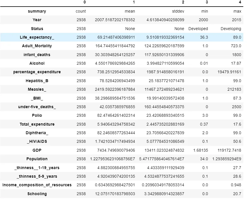
Descriptive Analysis of data

sparkDF = sparkDF.drop(*[‘Country’])
sparkDF.describe().toPandas().transpose()

Feature importance

We have columns which are positively correlated and negatively correlated, but we are considering all features for our prediction initially.

We would be doing further analysis and EDA on the data in upcoming posts.

corrs = []
columns = []
def feature_importance(col, data):
    for i in data.columns:
        if not( isinstance(data.select(i).take(1)[0][0], six.string_types)):
            print( “Correlation to Life_expectancy_ for “, i, data.stat.corr(col,i))
            corrs.append(data.stat.corr(col,i))
            columns.append(i)feature_importance(‘Life_expectancy_’, sparkDF)corr_map = pd.DataFrame()
corr_map[‘column’] = columns
corr_map[‘corrs’] = corrs
corr_map.sort_values(‘corrs’,ascending = False)

Modelling

We are using Databricks feature mlflow which is used to monitor spark jobs, model training runs and securing the results.

with mlflow.start_run(run_name=’StringIndexing and OneHotEcoding’):# create object of StringIndexer class and specify input and output column
    SI_status = StringIndexer(inputCol=’Status’,outputCol=’Status_Index’)sparkDF = SI_status.fit(sparkDF).transform(sparkDF)# view the transformed data
    sparkDF.select(‘Status’, ‘Status_Index’).show(10)# create object and specify input and output column
    OHE = OneHotEncoder(inputCol=’Status_Index’,outputCol=’Status_OHE’)# transform the data
    sparkDF = OHE.fit(sparkDF).transform(sparkDF)# view and transform the data
    sparkDF.select(‘Status’, ‘Status_OHE’).show(10)

Linear Regression

from pyspark.ml.feature import VectorAssembler# specify the input and output columns of the vector assembler
assembler = VectorAssembler(inputCols=[‘Status_OHE’,
‘Adult_Mortality’,
‘infant_deaths’,
‘Alcohol’,
‘percentage_expenditure’,
‘Hepatitis_B’,
‘Measles_’,
‘_BMI_’,
‘under-five_deaths_’,
‘Polio’,
‘Total_expenditure’,
‘Diphtheria_’,
‘_HIV/AIDS’,
‘GDP’,
‘Population’,
‘_thinness__1-19_years’,
‘_thinness_5-9_years’,
‘Income_composition_of_resources’,
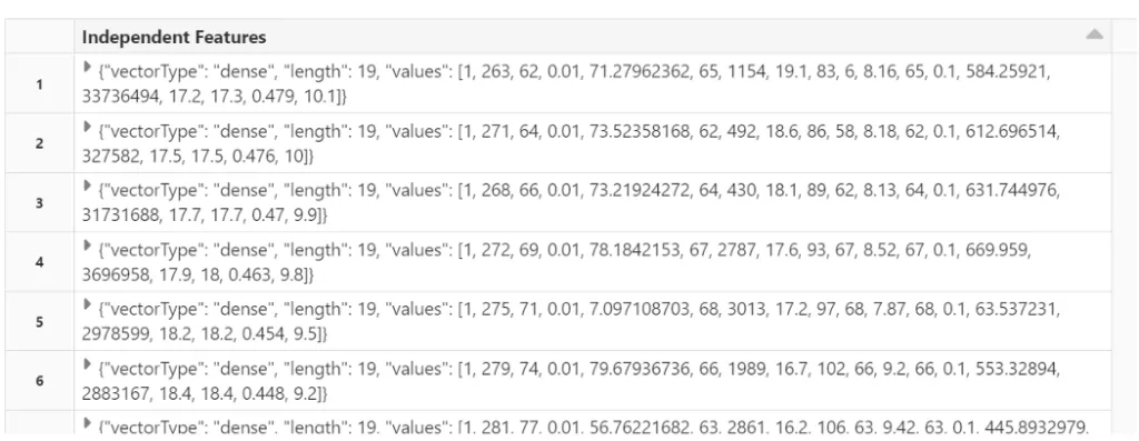
‘Schooling’],outputCol=’Independent Features’)# transform the data
final_data = assembler.transform(sparkDF)# view the transformed vector
final_data.select(‘Independent Features’).show()

Split the data into train and test

finalized_data=final_data.select(“Independent Features”,”Life_expectancy_”)
train_data,test_data=finalized_data.randomSplit([0.75,0.25])

In the training step we are implementing ML flow to track the training runs and it stores the metrics, so we can compare multiple runs for different models.

with mlflow.start_run(run_name=’Linear Reg’):
    lr_regressor=LinearRegression(featuresCol=’Independent Features’, labelCol=’Life_expectancy_’)
    lr_model=lr_regressor.fit(train_data)

    print(“Coefficients: ” + str(lr_model.coefficients))
    print(“Intercept: ” + str(lr_model.intercept))

    trainingSummary = lr_model.summary
    print(“RMSE: %f” % trainingSummary.rootMeanSquaredError)
    print(“r2: %f” % trainingSummary.r2)

Output: Coefficients: [-1.6300402968838337,-0.020228619021424112,0.09238300657380137,0.039041432483016204,0.0002192298797413578,-0.006499261193027583,-3.108789317615403e-05,0.04391511799217852,-0.0695270904865562,0.027046130391594696,0.019637176340948595,0.032575320937794784,-0.47919373797042153,1.687696006431926e-05,2.1667807398855064e-09,-0.03641714616291695,-0.024863209379369915,6.056648065702587,0.6757536166078358] Intercept: 56.585308082800374

RMSE: 4.034376

r2: 0.821113

RMSE gives us the differences between predicted values by the model and the actual values. However, RMSE alone is meaningless until we compare with the actual “Life_expentancy_” value, such as mean, min and max. After such comparison, our RMSE looks pretty good.

train_data.describe().show()

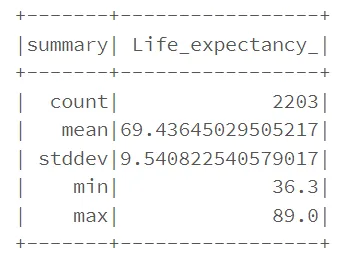
R squared at 0.82 indicates that in our model, approximate 82% of the variability in “Life_expectancy_” can be explained using the model. This is in align with the result. It is not bad. However, performance on the training set may not a good approximation of the performance on the test data.

#Predictions #RMSE #R2
with mlflow.start_run(run_name=’Linear Reg’):
    lr_predictions = lr_model.transform(test_data)
    lr_predictions.select(“prediction”,”Life_expectancy_”,”Independent Features”).show(20)

    lr_evaluator = RegressionEvaluator(
        labelCol=”Life_expectancy_”, predictionCol=”prediction”, metricName=”rmse”)
    rmse = lr_evaluator.evaluate(lr_predictions)
    print(“Root Mean Squared Error (RMSE) on test data = %g” % rmse)
    lr_evaluator_r2 = RegressionEvaluator(
        labelCol=”Life_expectancy_”, predictionCol=”prediction”, metricName=”r2″)
    print(“R Squared (R2) on test data = %g” % lr_evaluator_r2.evaluate(lr_predictions))
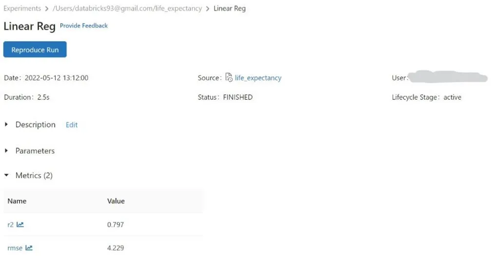
    #Logging Metrics using mlflow
    mlflow.log_metric(“rmse”, rmse_lr)
    mlflow.log_metric(“r2”, r2_lr)

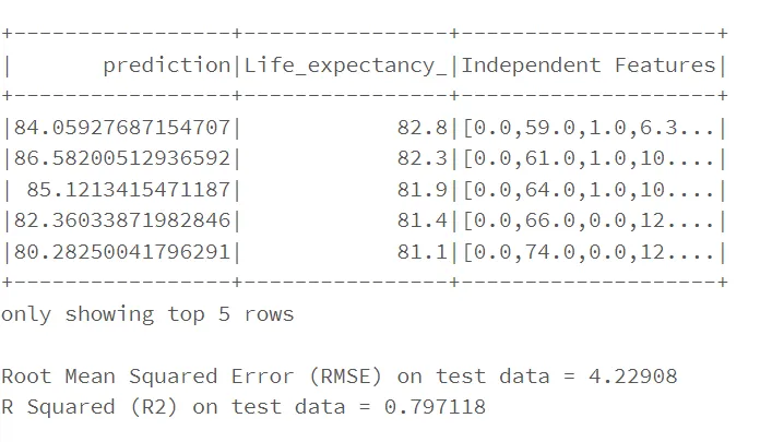
RMSE and R2 for the test data are approximately same in comparison to train data.

mlflow logging for rmse and r2 for Linear Reg model,

Decision Tree

from pyspark.ml.regression import DecisionTreeRegressor
with mlflow.start_run(run_name=’Decision Tree’):
    dt = DecisionTreeRegressor(featuresCol =’Independent Features’, labelCol = ‘Life_expectancy_’)
    dt_model = dt.fit(train_data)
    dt_predictions = dt_model.transform(test_data)
    dt_evaluator = RegressionEvaluator(
        labelCol=”Life_expectancy_”, predictionCol=”prediction”, metricName=”rmse”)
    rmse_dt = dt_evaluator.evaluate(dt_predictions)
    print(“Root Mean Squared Error (RMSE) on test data = %g” % rmse_dt)

    dt_evaluator = RegressionEvaluator(
        labelCol=”Life_expectancy_”, predictionCol=”prediction”, metricName=”r2″)
    r2_dt = dt_evaluator.evaluate(dt_predictions)
    print(“Root Mean Squared Error (R2) on test data = %g” % r2_dt)
    mlflow.log_metric(“rmse”, rmse_dt)
    mlflow.log_metric(“r2”, r2_dt)

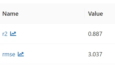
Output: Root Mean Squared Error (RMSE) on test data = 3.03737, Root Mean Squared Error (R2) on test data = 0.886899

Both RMSE and R2 are better than Linear Regression for Decision Tree.

Metrics logged using mlflow,