DMN, Meet Machine Learning

Blog: Method & Style (Bruce Silver)

While DMN adoption continues to accelerate, we can only admire the current frenzied interest in machine learning. Both technologies are trying to do similar things – make decisions – but they go about it in very different ways. DMN, which evolved from business rules and, before that, expert systems, is based on intuitive understanding of the logic. Decision modelers are assumed to be subject matter experts. On the other hand, machine learning – formerly called predictive analytics or data mining and now marketed as “AI” – assumes no intuition about the underlying logic, which is based instead on the statistics of past experience. Machine learning modelers are typically not subject matter experts but data scientists, trained in applied mathematics and programming. Because the language of machine learning is technical, few decision modelers know that much about it. This post will serve as a brief introduction.

Transparent vs Opaque Logic

You often hear that the logic of DMN models is explainable or transparent but the logic of machine learning models is opaque, a black box. Decision tables are really the most explainable part of DMN. Their logic is simple because decision table inputs are typically not raw input data but refined high-level features provided as supporting decisions. The top levels of a DRD are thus often decision tables while the bottom levels consist of all manner of value expressions that refine the input data into those high-level features. In contrast, machine learning algorithms, lacking intuition about what the high-level features should be, operate on the raw data directly. This further contributes to the opacity of the logic. We are primarily interested in so-called supervised learning models, which are “trained” on a large number of examples, each containing values of various attributes or “features” and having a known outcome. In training, the model parameters are adjusted to maximize the prediction accuracy. The trained model is then used to predict the outcome of new examples.

As machine learning gains influence on day-to-day decision-making, its inability to explain the reasons for its decisions is increasingly seen as a problem. One answer to the demand for “explainable AI” is DMN and machine learning working together. Although little explored to date, this can occur in a couple different ways:

Machine learning can be used in supporting decisions to refine raw input data into the high-level features used in decision tables. Even though the machine learning decision logic may be opaque, the top-level decision logic is transparent.
Some machine learning models can be transformed into DMN models, revealing hidden relationships in the data. This adds intuition to the decision logic which can be fed back to the machine learning model in the form of additional refined attributes. The result is often simpler models and more accurate prediction.

In this post we’ll see both of these at work in a customer retention scenario at a wireless carrier.

DMN Can Execute Machine Learning Models

You may not realize it, but the ability to execute machine learning models is a standard feature of DMN. From the start, the DMN spec said that in addition to the normal value expressions modeled in FEEL, decisions can execute machine learning models packaged using the Predictive Model Markup Language, or PMML. PMML, administered by the Data Mining Group, is not a marchine learning algorithm but a common XML format encompassing a wide variety of machine learning algorithms, including decision trees, logistic regression, support vector machine, neural networks, and others. By providing a standard format for a wide range of machine learning model types, PMML enables interchange and interoperability across tools. That means the tool or platform used to execute a machine learning model – for example, a DMN tool – does not need to be the same as the one used to create it. Although Trisotech does not create PMML models, its DMN Modeler can execute them. In this post we’ll see how that works and how DMN can be used to make machine learning human-understandable.

DMN’s mechanism for incorporating PMML is as an external function BKM. In addition to a FEEL expression, the spec says a BKM’s logic may be an external function, either a Java method or a PMML model. Trisotech DMN Modeler supports PMML execution in this way.

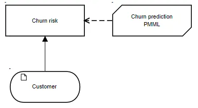
To illustrate this, consider the scenario of a wireless carrier trying to retain a customer at risk of “churn”, meaning switching to a new carrier. The decision model is shown below:

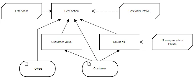
The input data are Customer, with attributes taken from billing records, and Offers that could be extended in order to retain the Customer. The DMN decision Churn risk executes the machine learning model Churn prediction PMML, returning a Boolean value. If Churn risk is true, the decision Best action invokes a second machine learning model Best offer PMML that suggests the Offers likeliest to be attractive to this Customer. Supporting decision Customer value computes a value metric for retaining this Customer and for each Offer, the BKM Offer cost computes its cost. Based on these inputs, Best action selects an Offer, its decision logic explainable even if the logic of Churn prediction PMML and Best offer PMML is not.

Churn Prediction

To illustrate how DMN and PMML work together, we will focus on Churn risk and Churn prediction PMML. The example is an adaptation of a sample app supplied with the open source machine learning tool Knime. The machine learning data is taken from the billing records of Customers who contacted the carrier with an issue. The table below is a fragment of a file containing over 3000 examples. Column 8 “Churn” is the output, with the value 1 if the Customer did not renew the carrier agreement (Churn = true) or 0 if he did renew (Churn = false). The other columns serve as inputs to the machine learning model. Already you see one basic difference between machine learning and DMN: Machine learning models typically operate directly on the raw data found in systems of record, whereas DMN typically refines that data in supporting decisions before making the final decision.

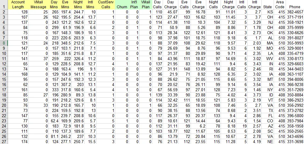
The goal of the machine learning model is to predict, for a new Customer, whether he is likely to churn. And here is a second difference from DMN: The modeler starts with little or no intuition about what combination of these Customer attributes will predict churn. But the machine learning model does not depend on intuition. You just feed it enough examples from past experience and it figures it out.

There are a variety of machine learning algorithms that could be applied to this problem. Some, like logistic regression or support vector machine, find the combination of numeric coefficients that, when multiplied by Customer attributes and summed, best predict churn. (Note: This is why machine learning often models Boolean inputs like VMail Plan as numbers, either 0 or 1.) Others, like decision tree, define a sequence of yes/no tests, each on a single Customer attribute, that best separate churn from no-churn examples. This branching is continued until there are very few examples on a branch, at which point the majority output value becomes the prediction for the branch. Decision trees are especially interesting for DMN, because the resulting tree model can be converted to a decision table, which can be inspected and its logic understood.

Measuring Machine Learning Accuracy

The goal of any machine learning model is maximum prediction accuracy, but what does that really mean? Like many decision models, the outcome of this one is binary, either churn or no-churn. If we call churn “positive” and no-churn “negative” and we call the prediction true if the predicted value matches the actual value, we have the following possible outcomes for each prediction: true positive (TP), true negative (TN), false positive (FP), and false negative (FN).

The metric accuracy is defined as (TP + TN)/(TP + FP + TN + FN), but this is not necessarily the most important measure when the examples are highly skewed, meaning many more negatives than positives. Precision, defined as TP/(TP + FP), measures what fraction of predicted positives are actual positives. Recall, defined as TP/(TP + FN), measures what fraction of actual positives are predicted. The metric you are trying to optimize – or perhaps some combination of these – depends on the circumstances of the decision. The four numbers TP, TN, FP, and FN, comprising the model’s confusion matrix, are provided by the tool used to create the model.

Actual / Predicted	0	1
0	TN	FP
1	FN	TP

Creating the Machine Learning Model

For this scenario, the machine learning model was created using a free open source tool called Knime. Most machine learning models are created by programmers in Python or R, but Knime is nice for non-programmers because models can be created simply by assembling graphical widgets in a workflow.

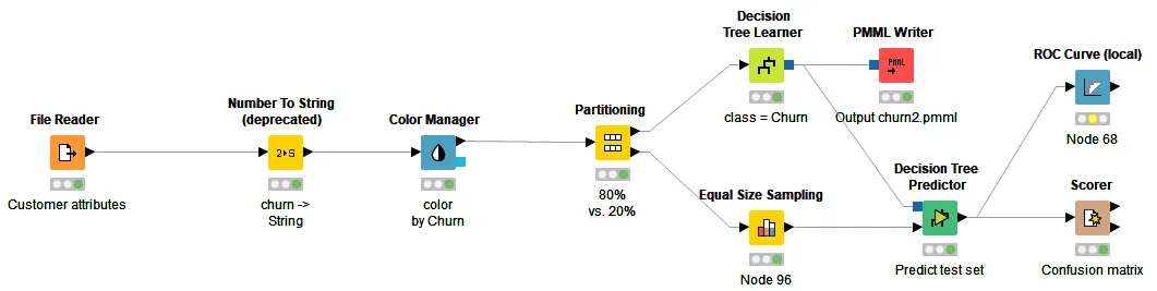
Here the File Reader node ingests the Excel file of Customer attributes. The Partitioning node randomly splits the examples into a training set (80%) and test set (20%). This is important for any type of machine learning model but especially important for decision trees, which are prone to “overfitting”. Overfitting gives high accuracy on the training set but degraded accuracy on untrained examples. For this reason, you train the model on the training set examples but measure accuracy on a separate test set, called cross-validation. The Equal Size Sampling node ensures that the test set has an equal number of churn and no-churn examples. The Decision Tree Learner node trains the decision tree. This is passed to the Decision Tree Predictor node, which applies it to the test set examples. The Scorer node reports the confusion matrix for the test set. The PMML Writer node creates a PMML file for the model.

One way to control overfitting in decision trees is to increase the minimum number of examples on a branch. When the branch contains fewer examples than that, no more splitting of the branch is allowed. Using the Knime app’s original value of 6 (out of a total of 194 examples in the test set), the Scorer node reports the following confusion matrix:

Actual / Predicted	0	1
0	91	6
1	26	71

Accuracy 83.5%, Precision 92.2%, Recall 73.2%

Gradually increasing the minimum number of examples on a branch leads to an optimum value of 10, with the improved confusion matrix below:

Actual / Predicted	0	1
0	93	4
1	24	73

Accuracy 85.6%, Precision 94.8%, Recall 75.3%

Executing the PMML

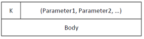
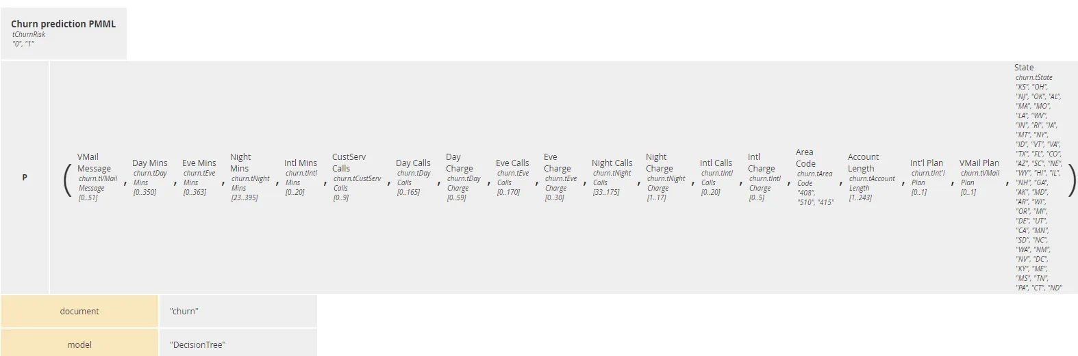
This model was saved as churn.pmml. Trisotech DMN Modeler is able to invoke PMML models and use the returned result within the decision logic. (Note: This requires the PMML subscription feature. Contact Trisotech for details.) As mentioned earlier, DMN functions – typically BKMs – by default use FEEL as their expression language, but the spec also allows them to be externally defined as either Java methods or PMML models. A PMML-based BKM is distinguished by the code P in the Kind cell of its boxed expression, displayed to the left of its list of parameters:

The parameters of the BKM are the inputs (DataFields) specified in the PMML model. The PMML DataField denoted as “predicted” is the BKM output.

The Body cell of a PMML BKM is always a context with the following two context entries:

document, specifying the imported PMML filename
model-name, the name of a model in the imported file

In DMN, a decision invokes this BKM in the normal way, passing parameter values and receiving back the BKM result. A PMML model must be imported into DMN before it can be invoked.

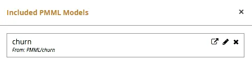
In the DRD shown here we have a decision Churn risk invoking BKM Churn prediction PMML, both type tChurnRisk, with allowed values 0 and 1 to match the PMML DataField Churn. Now, on the DMN ribbon (assuming you have the PMML feature enabled in your subscription), click on the PMML icon to upload churn.pmml to a repository in your workspace.

Then click the icon again and Add the PMML model to your DMN model. Adding a PMML file works like the Include button for normal DMN import. The PMML is imported in its own namespace, which is referenced as a prefix to the names of any imported variables and types. Trisotech DMN defaults the prefix to the name of the imported model – in the figure below it is churn – but using the pencil you can edit it to something else if you like.

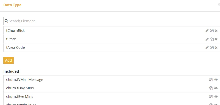
Datatypes

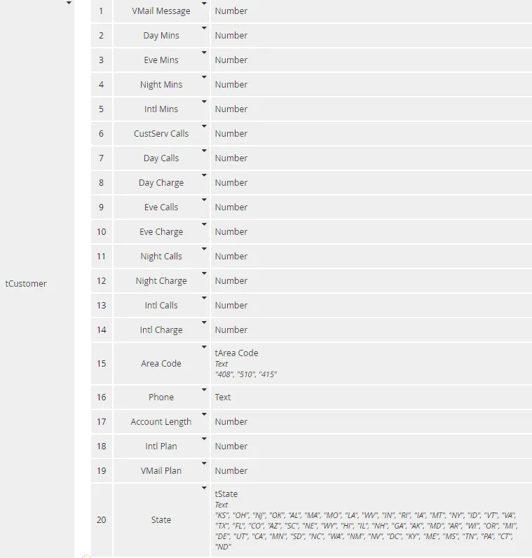
PMML has its own type system, which is slightly different from FEEL, but on PMML import Trisotech automatically creates a corresponding FEEL type for each input (PMML DataField) that is not a simple base type. The created types are namespace-prefixed, as mentioned. You need to convert them to non-imported types, but this is simply done by clicking the copy/paste icon for each one. In this model most inputs are numbers, but because Knime reports their minimum and maximum values in the dataset, Trisotech creates item definitions for them with these constraints. Actually, we’d rather not have these constraints, as it’s possible a new test case could have an input value outside of the range or the original dataset. We can simplify the model by eliminating those item definitions in favor of the FEEL base type Number. The only ones we need to keep are the enumerations tAreaCode and tState.

Finally we need to add the structure tCustomer describing our input data element, with one component per input DataField in the PMML, and assign it to input data Customer:

Modeling the BKM

Returning to the DRD, we now define the decision logic for the BKM Churn prediction PMML, a context. Changing the default Kind code F (for FEEL) to P (for PMML) automatically creates the context entries document and model. Clicking in the right column automatically extracts values for those entries from the included PMML file.

Invocation

The decision Churn risk invokes the BKM. Selecting Invocation as the expression type makes the mapping trivial:

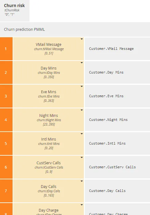
And that’s all you need to do. Now you are ready to execute the model.

Execution/Test

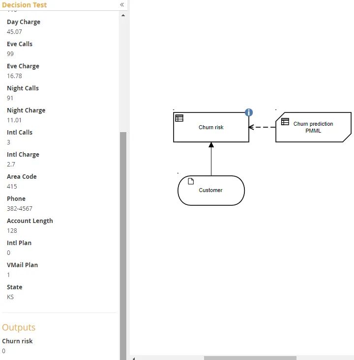
As with any decision model, running it in Execution/Test will reveal any problems. In the Execution/Test dialog, I manually entered values from the first row of the Customer attribute spreadsheet shown earlier. On execution it returns the predicted value 0, which matches the actual value from the spreadsheet (Churn, column 8). At this point you could deploy the model as a DMN decision service.

Going Further with DMN

What we’ve seen so far is that you can take a PMML model created in a third party tool and execute it as a BKM in a DMN model. That’s impressive, but we haven’t seen yet how DMN makes the PMML logic more explainable. To get some idea of the logic, you could scrutinize the PMML file and draw the decision tree as a BPMN flow with gateways. That’s not only a lot of work but the result is not so easy to understand. A much better way is to convert the decision tree into a DMN decision table. Again, you could do this by hand, but it’s easier to write a program to do it.

The results are quite enlightening. Here is a fragment of the table created from churn.pmml:

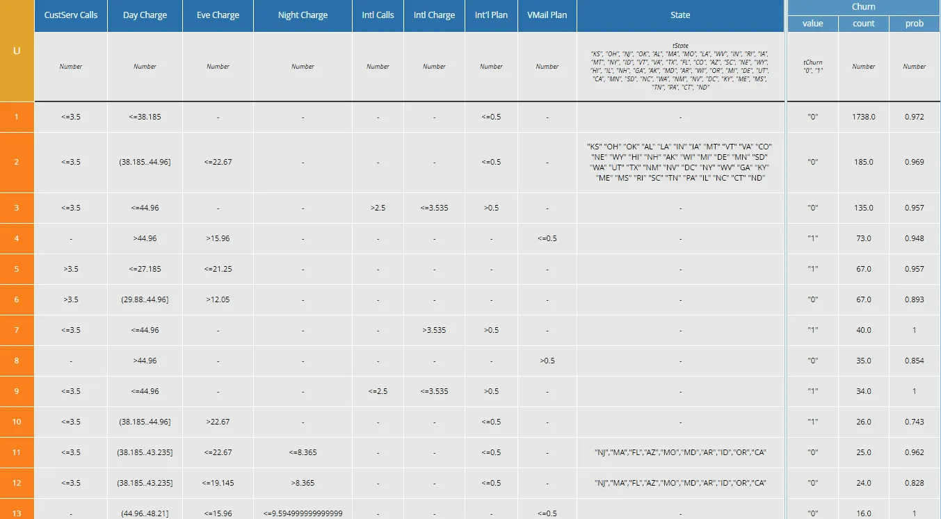
The full decision table has 21 rules, and my program has sorted them in order of counts in the training set to see which rules are matched most often. Recall there were 20 inputs in the original PMML, but only 9 of them are involved in the actual decision logic. Columns for the unused inputs have been deleted from the table. (The original PMML model, with a minimum of 6 examples per branch, resulted in a table with 10 inputs and 37 rules, a table with twice as many cells but less accurate on the test set!)

We can examine this table to try to understand the reasons why a Customer will churn. From rule 4 above, a high Day Charge and Night Charge looks like one factor. From rule 5 and others, we see that a high number of Customer Service Calls is another factor. From rule 7, a high International Charge looks like a factor, and from rule 9 an International Call Plan but low International Charge looks like another factor. On the other side, it looks like Customers with a Voice Mail plan are not likely to churn. All of these make some sense intuitively.

Feeding Back Intuition to the Machine Learning Model

My takeaway from looking at this table was that perhaps we should consider the sum of Day, Evening, and Night Charges as an additional “refined” input, also the average cost per International call. State doesn’t make a lot of sense to me, so let’s get rid of that one. I went back to the Customer attribute spreadsheet, eliminated the unused inputs (plus State) and added the refined inputs Total Charge and International Charge per call. Then I created a new decision tree with Knime using the revised spreadsheet and converted that to a decision table, just to see if it made any difference.

It did. Not only is the new model more accurate…

Actual / Predicted	0	1
0	95	2
1	19	78

Accuracy 89.2%, Precision 97.5%, Recall 80.4%

… but it is simpler and easier to interpret:

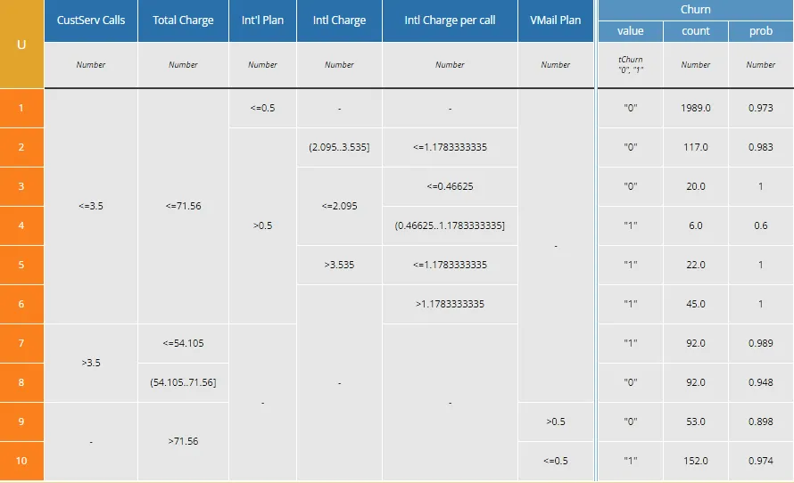
Once the Total Charge input was added, the Day Charge, Eve Charge, and Night Charge columns dropped out. Now the table has just 6 inputs and 10 rules.

My intuition from examining the earlier decision table was confirmed. Factors leading to churn include high Total Charge, high number of Customer Service Calls, and high International Charge per call. Having a VoiceMail plan discourages churn. Armed with this data, the carrier can make more informed decisions about what type of retainment offers to make and possibly changes in their pricing policies.

The accuracy of this model is surprisingly good, given that we started with zero intuition about the factors suggesting churn risk. A full 97.5% of Customers predicted to churn actually did in the test set. Recall is more difficult, but over 80% of Customers that churned were predicted by this model. Now that we have a better idea of the significant inputs, we could go back and use them in a different machine learning model – say, logistic regression or SVM, which often have higher accuracy than decision trees – and see if we can do even better.

The bottom line is that while machine learning is doing just fine on its own, integrating it with DMN can not only add explainability but actually improve accuracy.

The post DMN, Meet Machine Learning appeared first on Method and Style.