---

Disco 2.0

It is our pleasure to announce the immediate release of Disco 2.0!

There are many changes and improvements in this release, most of which were informed by your suggestions and feedback. But the marquee feature of Disco 2.0 is TimeWarp, which allows you to incorporate business days and working hours into your process mining analysis.

Being able to specify working days and working hours must be one of the most frequently requested features that we have received for Disco so far. With Disco 2.0, we now make it possible to include working days and working hours into your process mining analysis in the most humane way. We are super excited about TimeWarp, and we can’t wait to hear about what you will do with it!

Disco will automatically download and install this update the next time you run it, if you are connected to the internet. If you are using Disco offline, you can download and run the updated installer packages manually from fluxicon.com/disco.

To make yourself familiar with the TimeWarp functionality in Disco 2.0, you can watch the short video above. Please keep reading if you want the full details of what we think is a great update to the most popular process mining tool in the world.

The Trouble with Time

Support for business hours and holidays in Disco has been one of the most frequent requests we get from our customers. With TimeWarp, we think we have finally come up with the perfect solution to a tricky problem.

Unfortunately, time is a very human and, thus, kind of a messy construct. We have daylight savings time in many parts of the world, but everywhere it is handled in a different manner. There are leap years, and leap seconds, synchronizing our “official” notion of time with their astronomical references. And, to top it off, we have widely differing ideas about which days of the week, and which days of the year, are supposed to be “work days”, and when the office stays closed.

This means that a simple question like “How much time passed between 12 February and November 4” can have very different answers, depending on the year and the location in question. And if you would like the answer in business hours, it gets even more complicated. If you need the precise duration in every case, you will need to consider every exception and edge case, which can become very computationally expensive and slow at scale.

In Disco, we calculate a lot of durations for many purposes. They are the basis for the excellent performance analysis capabilities Disco provides, and power many more features like our best-of-breed mining algorithm. Since many of our customers use Disco with huge amounts of data, using a very precise but slow method of calculating durations is out of the question. Using a trivial but precise measurement method could have meant that a one-minute analysis would have turned into half an hour or more.

On the other hand, we really do want absolute precision for duration measurements. If you have only Monday through Friday as working days, simply multiplying every duration with 5/7 will be pretty fast, but it is also quite useless if you want to precisely measure SLAs.

With TimeWarp, we have found a way to square that circle. The duration measurement engine in TimeWarp is precise to the millisecond, while at the same time it is blazingly fast. There is no need for you as a user to make the trade-off between precision and performance, because you can truly have it all. This means that you can now perform business hours-aware performance analyses with Disco on huge data sets, with negligible impact on performance. We think you are going to love TimeWarp, as it keeps perfectly with the Disco tradition of providing guaranteed scientifically accurate results, reliably, with record speeds.

The Limitation of Calendar Days

When you look at Service Level Agreements (SLAs) in your organization, then you will see that many of them recognize that there are certain days on which people don’t work.

It would not be fair to consider a customer request that was initiated on Friday and answered on Monday in the same way compared to one that was raised on Monday and answered on Thursday. People recognize that their banks, insurance companies, municipalities, and other organizations have weekends, too. So, the weekends should not “count”.

But process mining evaluates the timestamps in your data set and, naturally, uses these timestamps to calculate all the performance metrics like case durations, waiting times, and other process-specific KPIs in calendar days.

For example, let’s look at the following credit application process. The internal SLA for the operational unit is 3 business days. This means that the time between the ‘Credit check’ activity and the outcome (which can be ‘Approved’ or ‘Rejected’, or ‘Canceled’ if the application was withdrawn by the customer) should not be longer than 3 days.

We can add a Performance filter to check this SLA in our process mining analysis (see below).

When we look at the result of the Performance filter then it appears as if 53 % of all cases lie outside of our SLA (see below).

But these 53% are based on measuring the case durations in calendar days, while the SLA that we want to measure is 3 business days. This is a big problem, because there are cases that actually meet the SLA in terms of business days but they appear in the 53% because there was a weekend in between. So, the true number of cases that meet the SLA is unknown.

SLAs are not only internal guidelines. For example, outsourced processes are managed through contracts that include one or more SLAs. There may be financial penalties and the right to terminate the contract if any of the SLA metrics are consistently missed. However, you cannot fully analyze a process with contractual SLAs in business days if all you can measure are calendar days.

The problem with the desire to measure business days in process mining is that you can’t really work around this problem in an easy way. You can’t change the timestamps, because the timestamps indicate when something truly happened.

You can calculate the business days outside of the process mining tool (typically, this involves programming). But you can do this only for a specific pair of timestamps, from which to which the time should be measured. However, the power of process mining comes from the ability to take different perspectives, and to be able to leave out activities to focus on the process steps that you are interested in in a flexible way. You completely lose that flexibility if you pre-calculate working days in your source data set.

So, what we have done with TimeWarp is to bring the ability to analyze your process based on business days and working hours right into Disco.

Let’s take a look at how this works!

Removing Weekends

To analyze the credit application process from above in business days, we need to remove the weekends.

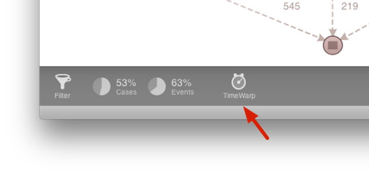
To do this, you can click on the new TimeWarp symbol in the lower left corner (see below).

You are then brought into the TimeWarp settings screen, where you can enable TimeWarp (see below).

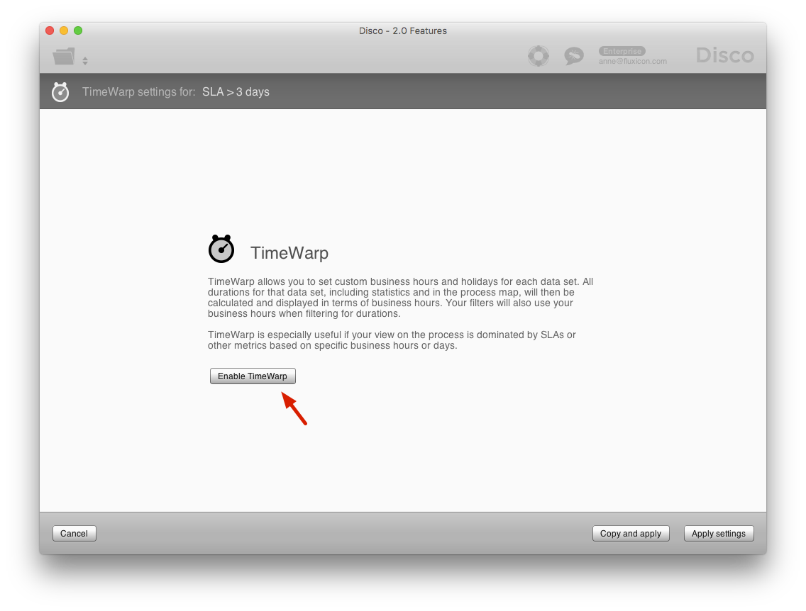
As soon as you have enabled TimeWarp, you will see the calendar view of a week – from Monday on the left to Sunday on the right. TimeWarp pre-fills the week days with a green working time period from 8am until 6pm and indicates Saturday and Sunday as closed. But you can change the TimeWarp settings to match your own working day requirements.

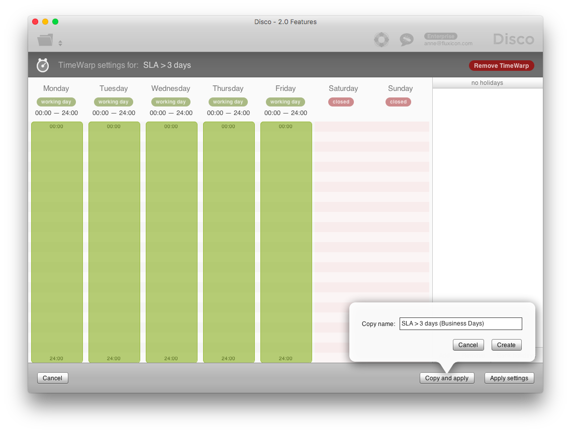
For example, to analyze the credit application process based on business days, all we want to do for now is to remove the weekends. As for the week days, we want to fully count them. So, we adjust the week day periods that should be counted by TimeWarp to stretch the whole day from midnight to midnight.

To adjust all week day periods at once, you can click and move the Monday timeframe. All the other week days will be adjusted accordingly (see below).

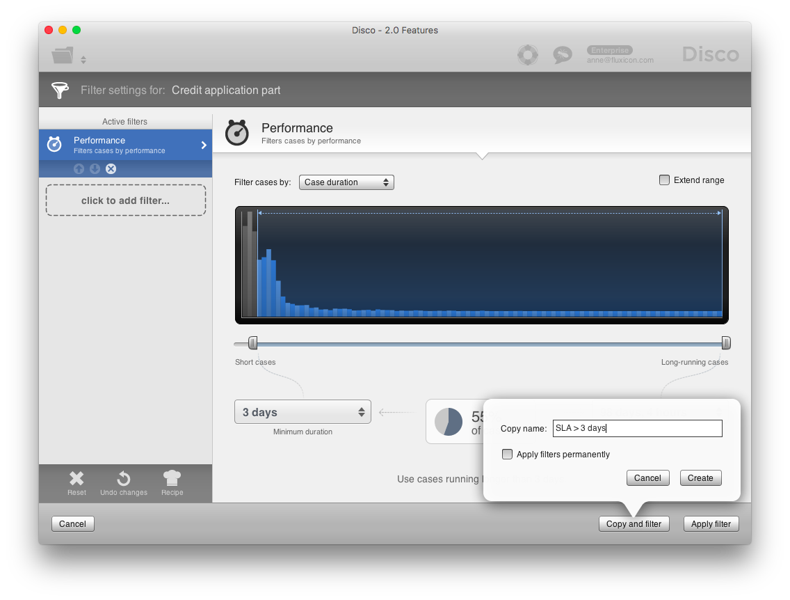
Now, we want to save this as a new analysis in our project, so that we can compare the outcome to the previous analysis. We click the ‘Copy and apply’ button and give the new analysis a short name that indicates that we are now measuring the SLA based on business days (see below).

After pressing the ‘Create’ button, we can now see that not 53% but just 41% of the cases are outside the SLA if we remove the weekends from our analysis!

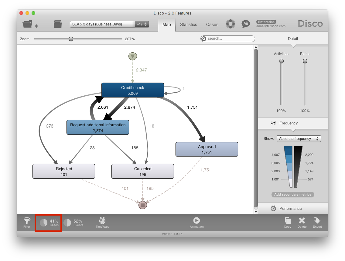
This is great, because we now have the true number for the SLA measurement. Furthermore, every case in our analysis result is truly in violation of the SLA, so the information that we provide to the process owner will be more actionable for them in their root cause analysis.

Removing Holidays

In fact, we need to do one more thing if we want to be precise: There are not only weekends but also public holidays on which people don’t work. These holidays should also not be counted in our SLA measurement.

We can easily add a holiday specification to our TimeWarp settings in the following way.

We click on the Timwarp symbol in the lower left corner again and then press the ‘Bank holidays’ button in the lower right. A list of countries will be displayed and we choose the Netherlands as the country from which we want to add the holiday specifications (see below).

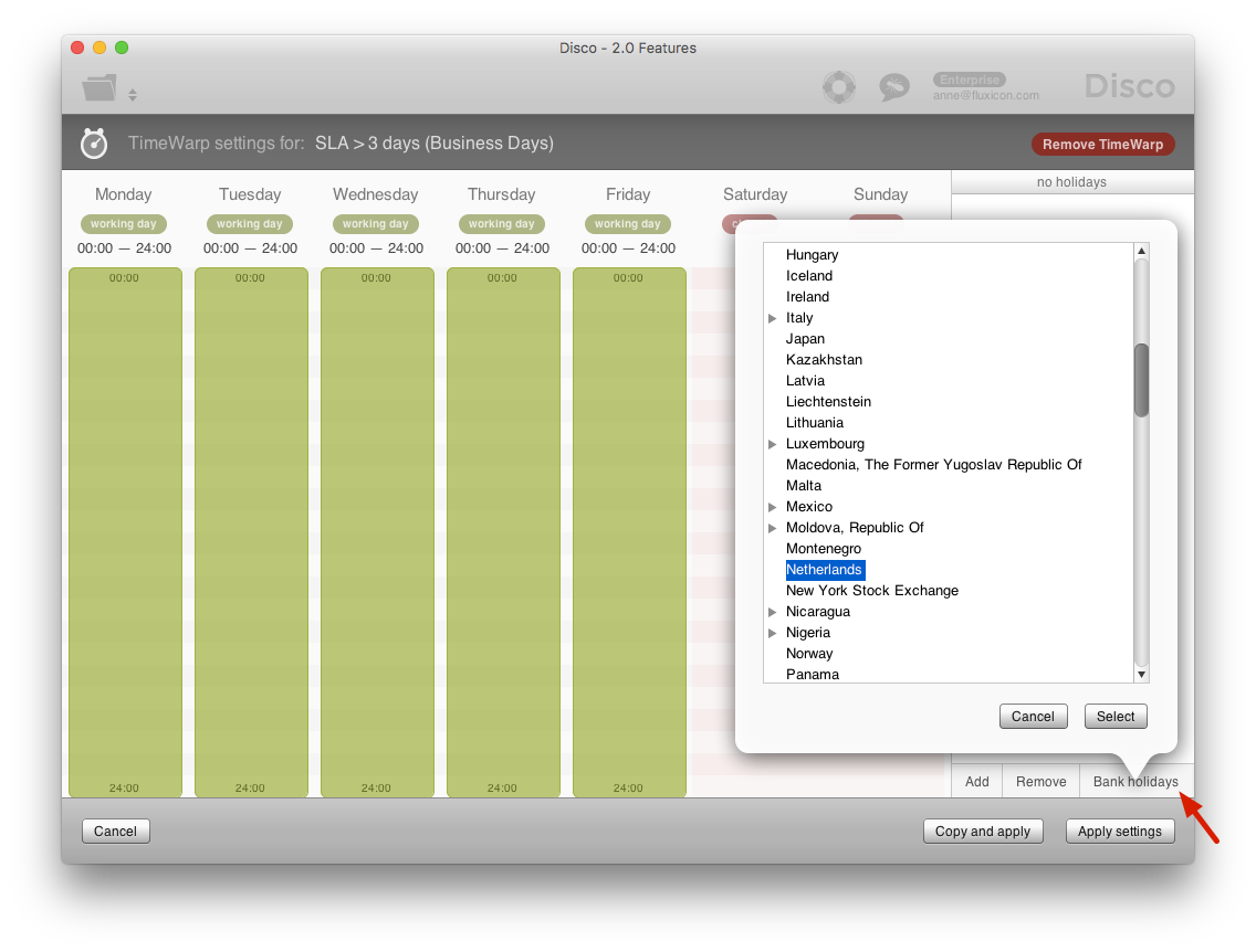
After we have pressed the ‘Select’ button, all holidays in the time period covered by our data set are added automatically to the list of holidays on the right. The data set that we are analyzing is covering the credit application process from February 2012 until June 2012. So, we can see that holidays such as the Easter holidays in this period have been added automatically (see below).

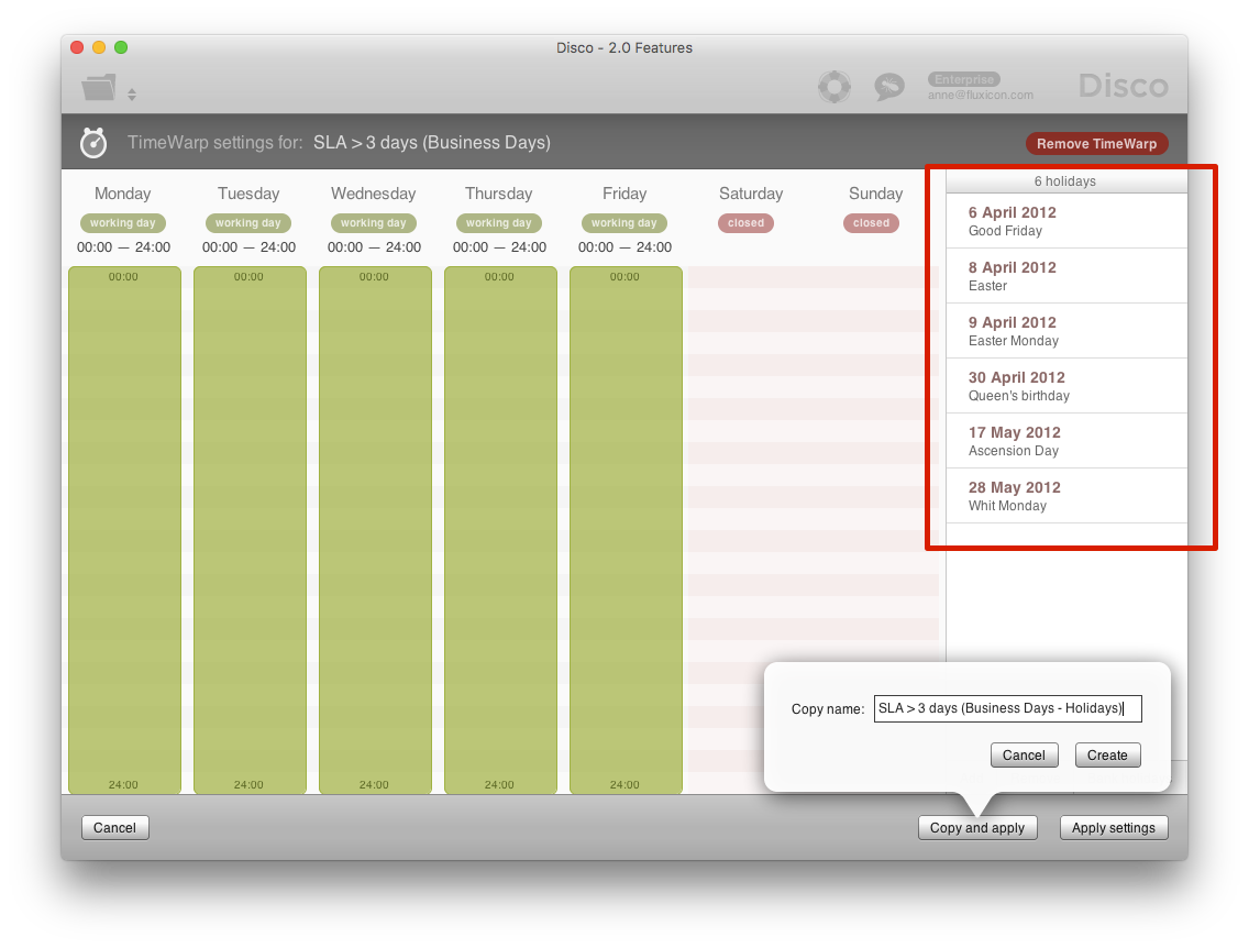
If your organization has some additional days that are free and should not counted, or if some of the public holidays in your region are actually a working days for your organization, you can also manually add and remove holidays right there, but the pre-populated list is a great start.

After you click the ‘Apply settings’ button, we can see that by removing the holidays from business day measurements, the number of cases that lie outside the SLA of 3 business days actually dropped to 40%. That’s a big difference to 53% from the initial calendar-day based measurement!

Analyzing Working Hours

Sometimes, you do not only want to remove weekends and holidays, but you actually want to take into account the working hours as well.

For example, in the front office part of the credit application process, customers can submit applications online and through the phone, and the ambition for the bank is to provide a fast initial response to the customer.

If we look at the durations in the process map, then we can see that it takes 29.3 hours on average between the call and the pre-approval (see below). The SLA for this part of the process is 8 working hours. However, like in the example above, the durations calculated by the process mining tool are based on calendar days.

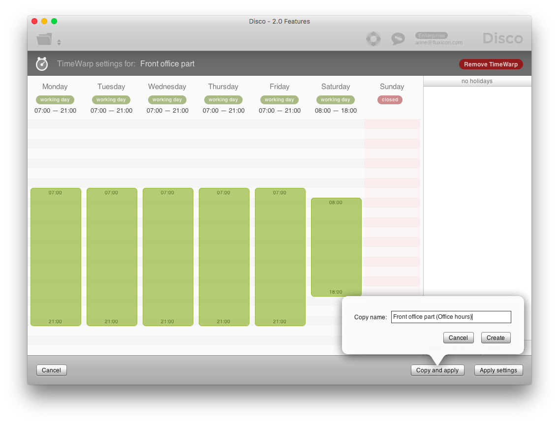
To take the working hours of the front office team into account, we enable TimeWarp for the data set. The front office team in the callcenter works from 7am to 9pm on weekdays and from 8am to 6pm on Saturdays. In the default settings, Saturdays are closed. But you can click on the ‘Closed’ badge at the top to include a weekend day as a working day (see below).

We then continue to set the right time table to indicate the right working hours of the different days of the week for the callcenter team in the front office (see below).

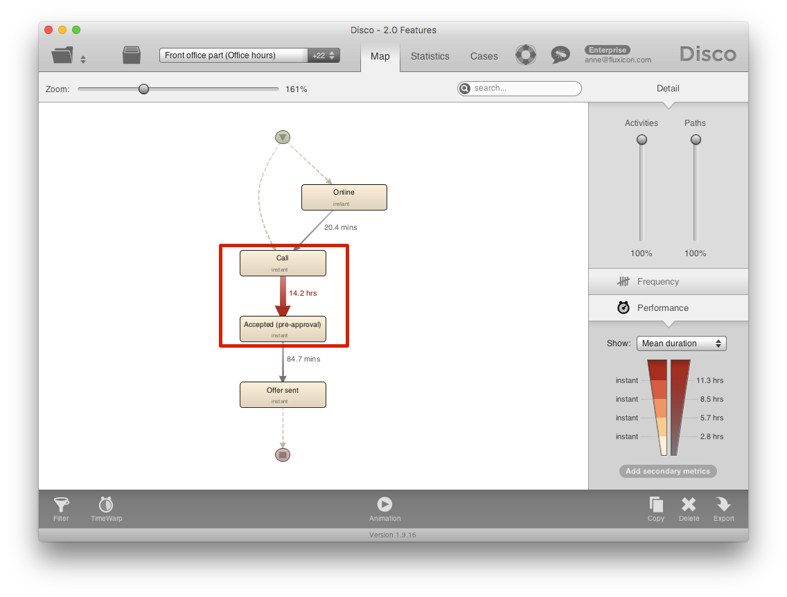
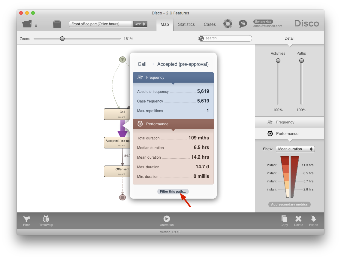
We can see that the average durations in the process map have changed (see below). Instead of 29.3 hours it just takes 14.2 hours on average between the call and the pre-approval. The average times have changed, because times between shifts (for example, between 9pm of a weekday and 7am of the next weekday) are not counted.

This is now the right basis for our SLA analysis. To check how many cases take more than 8 working hours between the call and the pre-approval, we can simply click on the path in the process map and use the shortcut ‘Filter this path…’ to add a pre-configured filter (see below).

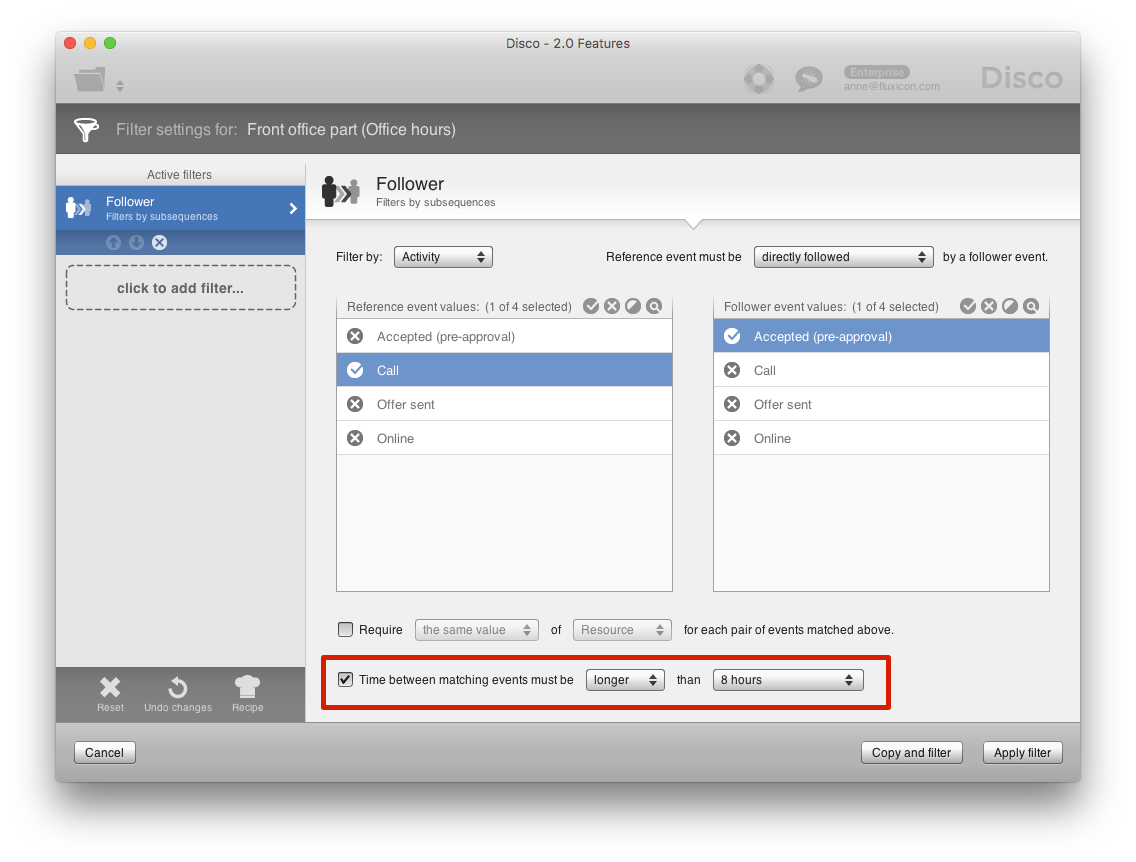
In the Follower filter that was automatically added to our data set we can add an in-process SLA by enabling the ‘Time between events’ option. We set the filter setting to ‘longer than 8 hours’ to indicate that we are interested in all cases that are not meeting our SLA (see below).

Disco will now automatically take our working hour specification into account to filter the data set based on the 8 working hours SLA. After applying the filter, we can see that 46 % of the cases do not meet our 8 working hours SLA (see below).

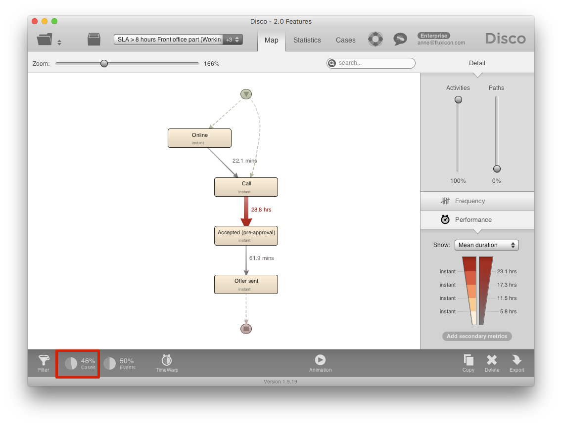
The working hours that we configured for the different weekdays in TimeWarp are essential to perform this SLA analysis on the right basis. If we would remove the TimeWarp settings for this data set again, we would see that ca. 10 % more cases would be included in our filter result as a false positive.

For example, if a call came in at 8:30pm on a Friday and the offer was ready at 7:30am on Saturday, then without TimeWarp this would be counted as 11 hours (above the 8 hour SLA limit). However, with the right TimeWarp settings enabled, it will be correctly counted as just 1 hour!

Full Transparency for Your Analysis Process

In addition to the new TimeWarp functionality, there are also some changes and additions that will be very useful for all process mining analysts but that are particularly exciting for auditors.

As an auditor, you have the requirement that you need to generate an audit trail for your analysis. This means that there should be a way to fully document all the steps that you have taken, so that other people are able to follow your steps and repeat your analysis. Since Disco 1.9, auditors already have an audit trail with the Audit report export in Disco. But in Disco 2.0 we take the traceability one step further.

You can now fully document how you arrived at your analysis result from the source data to the end result in addition to saving your project files with the full Disco workspace.

1. Import configuration

When you import your data set into Disco, you can choose a process perspective. And in many situations, you will actually look at your process from different angles.

To keep track of the perspective that you have chosen during the import, you previously had to manually document which columns were configured as Case ID, Activity, Timestamps, etc. Disco 2.0 now does this for you by adding the import configuration settings to the ‘Notes’ section of you data set (see below)

2. Permanent filters

When you clean your data set of data quality issues, or focus on a part of the process as a new baseline, you use the ‘Apply filters permanently’ option in the ‘Copy and filter’ settings (or the ‘Copy’ settings of your data set). As a result, all the filters will be applied but the outcome of the filtering step will be available as a clean, new data set and the percentage will be re-set to 100%.

However, sometimes it is important to keep track of which filters were previously applied in a permanent way to keep the full visibility of how you arrived at a certain analysis from the source data.

Disco 2.0 now adds the summary of the permanently applied filter settings to the end of your ‘Notes’ section in the data set as well (see below). The notes are also included in the audit trail export, so that you have all the steps from your import settings and all the filter steps documented along with any personal notes that you add during your analysis there.

3. Empty data sets as first-class citizen

Sometimes, the data set result after applying a filter configuration will be empty. And this can be a good thing. For example, if you are checking a Segregation of Duty rule for your process, then it is good if such a violation never occurred!

You could already export the audit report for empty filter results before, but now Disco will keep the data set in your workspace along with all other analyses. This way, you can document all your analyses in one place – even if some of them resulted in an empty data set (see below).

4. Export (or delete) multiple data sets at once

When you wanted to document your analyses outside of Disco, then you previously had to export the results for every analysis separately.

With Disco 2.0 you can now select multiple data sets and export, for example, all the PDF process maps, or the audit reports, for all the selected data sets at once (see below). This can also be handy if you want to clean up your workspace and want to delete multiple data sets that you don’t need anymore. They can now be all deleted with one click.

Filter Variants and Cases from the Cases View

Finally, people love the interactivity of Disco and the many short-cuts from the process map and statistics view that make your analysis so fast and productive (see this article on the Disco 1.9 release for an overview of the most important short-cuts).

We frequently heard from you that you would like to have these short-cuts also in the Cases view to quickly filter variants and cases right from there. Disco 2.0 now makes this possible. Simply right-click on the variant, or the case, that you want to filter for and use the short-cut (see below).

Other changes

The Disco 2.0 update also includes a number of other features and bug fixes, which improve the functionality, reliability, and performance of Disco. Please find a list of the most important further changes below.

• CSV Import: Improved concatenation of activities and resources based on multiple attributes (columns).

• CSV Import: Extended error reporting for files where some timestamps could not be parsed.

• CSV Import: Fixed a problem where some tab-separated files were not correctly auto-detected.

• XES Import: Improved error reporting when loading XES files with structural problems.

• MXML Import: Improved error reporting when loading MXML files with structural problems.

• Excel Import: Fixed a problem where some Excel sheets with empty rows could not be loaded.

• Workspace: Improved safeguarding of general workspace data integrity, and provide more user-friendly workspace recovery in case of data corruption.

• Workspace: Migrated to a future-proof, more collision-resistant hashing algorithm to improve data integrety.

• Bug Fixes: This update fixes several minor issues and user interface inconsistencies.

Finally, we would like to thank all of you for using Disco! Your continued feedback is a major reason why Disco is the best, the fastest, and the most stable process mining tool there is. Please keep sending us your feedback, and help us make Disco even better!