Read Blog Post

Read Blog Post

Contributed on March 9, 2022

0

241

Combining Lean Six Sigma and Process Mining — Part II: Measure Phase

This is the 3rd article in our series on combining Lean Six Sigma and process mining. It focuses on how process mining can be applied in the Measure phase of the DMAIC improvement cycle. You can find an overview of all articles in the series here.

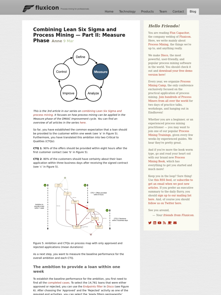
So far, you have established the common expectation that a loan should be provided to the customer within one week (see ‘a’ in Figure 5). Furthermore, you have translated this ambition into two Critical to Qualities (CTQs):

CTQ 1: 90% of the offers should be provided within eight hours after the first customer contact (see ‘b’ in Figure 5).

CTQ 2: 80% of the customers should have certainty about their loan application within three business days after receiving the signed contract (see ‘c’ in Figure 5).

Figure 5: Ambition and CTQs on process map with only approved and rejected applications (mean durations)

As a next step, you want to measure the baseline performance for the overall ambition and each CTQ.

The ambition to provide a loan within one week

To establish the baseline performance for the ambition, you first need to find all the completed cases. To select the 14,761 loans that were either approved or rejected, you can use the Endpoints filter in Disco (see Figure 6). After choosing the ‘Approved’ and the ‘Rejected’ activity as one of the required end activities, you can select the ‘Apply filters permanently’ option to reset the outcome of this filter as “the new 100%” of your data set.

Figure 6: Filtering approved and rejected loan applications to establish the baseline for the ambition

You can now measure the baseline performance for these loan applications to see how many are completed within seven days. To do this, you add a Performance filter and lower the upper case duration boundary to 7 days (see Figure 7). While configuring the filter, you already get an estimate of the number of cases covered by the current selection. After applying the filter, you can see in the final result that 9,782 cases (or 66% of the loan applications – see Figure 8) were actually completed within seven days.

Figure 7: Measuring the baseline for the ambition of completing loan applications within seven days

Note that if you had not reset the Endpoint filter result as your new base dataset using the ‘Apply filters permanently’ option, you would have measured your baseline performance for the initial data set of 20,732 cases. This initial data set would have included cases that were just started or are currently waiting for a reaction from the customer, etc., and not just the 14,761 cases that were either rejected or approved. The outcome would have been the same 9,782 cases, but the percentage would have been different because 9,782 cases are 47% of 20,732 cases. So, the baseline measurement % would not have been correct.

Figure 8: The resulting process map of all loan applications that were completed within seven days

Besides filtering the cases completed within seven days, you can also filter the cases that took longer than seven days (by inverting the selection of the Performance filter in Figure 7). While looking at these applications that took longer than seven days, you notice that the channel caused a big chunk of the delay. Sending the offer package by post and receiving it back from the customer per post adds two to four days to the lead time. Could this be one of the causes of the low conversion at this point in the process?

This finding triggered an interesting discussion. Moving the offline part of the application process to an online channel could significantly speed up the completion time. However, this would require a significant IT investment for the loan provider because they would need to extend the online platform to digitally sign the contract and securely provide the necessary documents for underwriting. And we are not in the improvement stage yet. Let’s keep focusing on measuring the baseline first.

CTQ 1: Offer provided within 8 hours

Establishing personal contact with the customer is an essential step in the process that is also highly valued by the customer. After the online application, the loan provider calls each customer to qualify their needs and provide them with the correct information.

Speed is considered one factor that influences the customer’s decision for a loan provider. Therefore, the management team had agreed that the offer should be provided within eight business hours after the first customer contact (CTQ 1).

CTQ 1 can be measured from the first activity of the process until the ‘Offered’ step. To create the baseline for this CTQ, you start from the entire data set again (not just the completed cases). You want to include the measurement for those cases that have not yet reached the end of the process, but an offer has already been made.

Figure 9: Cutting out the first part of the process (until the ‘Offered’ step) to measure the baseline for CTQ 1

To focus on this first part of the process, you can use the ‘Trim first’ option of the Endpoints filter (see Figure 9), again with the ‘Apply filters permanently’ option enabled to create the new baseline. The resulting process scope is now limited to just the first phase, which provides the correct basis for measuring the baseline for CTQ 1 (see Figure 10).

Figure 10: The resulting process scope for the baseline measurement of CTQ 1

Like measuring the ambition to provide a loan within one week, you can now use the Performance filter to measure how many offers the loan provider delivered within eight hours. The result is that for 3,175 of the 8,038 applications (39% of the cases), the customer service agent made an offer within eight hours.

However, in fact, this CTQ is defined in business hours. The customer contact center does not operate around the clock but six days a week. During weekdays they work from 8 am until 8 pm and from 8 am until 3 pm on Saturday. The non-working hours need to be excluded from the measurement. Otherwise, offers made for applications that came in shortly before the closing of the previous workday and completed immediately after the start of the next workday would (falsely) be measured as not meeting the CTQ.

To measure the baseline in business time as intended, you need to take one extra step: Using the TimeWarp functionality in Disco, you can define the call center team’s working hours. In addition to specifying the working times per day of the week, the holidays (which are whole non-working days) can be eliminated automatically (see middle in Figure 11).

The result is that you only count the “net” time in all the performance metrics. For example, the median time between the ‘Lead’ step (when the application reaches the call center) and the ‘Offer’ step (when the loan provider sends the offer out) changes from 18.6 (calendar) hours to 5.6 (working) hours. The time outside the team’s working time is not counted (see left and right in Figure 11).

Figure 11: The median performance measurements of the baseline process before and after adding the business hours and holidays using the TimeWarp functionality in Disco

The “net” time is also used for the performance statistics. For example, the case durations are now shown in pure working time as well. You could export these corrected business time durations from Disco (see Figure 12) and analyze the capability of the process by evaluating CTQ 1 in Minitab¹ (see Figure 13). It shows that a whole 56% (and not just 39% as was previously measured in calendar time) of the applications resulted in an offer within eight business hours. For 76% of the applications, the call center team could provide an offer within 16 business hours.

Figure 12: The case durations are also shown in business time after specifying the working hours with TimeWarp

Figure 13: The case durations can be exported from the process mining tool to be analyzed in Minitab

You can get the same results when you apply the Performance filter for up to eight hours case duration to the data set that has been corrected for the business time via TimeWarp in Disco itself (see Figure 14). So, it is unnecessary to go to Minitab for the measurement step. We can measure the CTQ directly in the process mining tool.

Figure 14: 56% of the cases meet the CTQ 1 of providing an offer within eight business hours

In addition to the actual measurement of the baseline, a further advantage of using the process mining tool is that you can analyze the process flows, variants, bottlenecks within the process, example cases, etc., in great detail. We will come back to using Minitab and Disco together in a complementary manner in the next phase of the DMAIC cycle.

CTQ 2: Decision within 3 business days

Finding the baseline for the underwriting process is a little bit more complicated. Especially defining the meaning of when exactly there is certainty about the loan is not so easy. After some deliberation, you decide to measure from the moment the applicants returned the signed contracts until the applications were either approved or rejected. To create this baseline, the Endpoints filter in ‘Trim’ mode can be used again as before (see Figure 15).

Figure 15: Creating the baseline for CTQ 2

When you measure the performance based on this baseline, you find that only 41% of the applications were approved or rejected within three days.

When you look further at the process, you find that something strange is happening: It should not be possible that incomplete applications are approved (see the highlighted path on the left side in Figure 16).
 Furthermore, you notice that the Work in Progress graph (via the ‘Active Cases over Time’ statistics) shows a significant drop every 22nd of the month (see highlighted drops on the right side in Figure 16). This means that a large number of cases are completed at the same time (in “bulk mode”).

Figure 16: Incomplete applications are approved (left), and sharp drops in the Work in Progress can be observed each 22nd of the month (right)

You are looking at some examples with the credit manager, and they can explain what happened: Besides the loan product, they also offer a credit product, for which some customers request to receive the payment on the 22nd of the month. In the IT system, the payout is connected to the activation of the loan. Therefore, these applications are (artificially) set into the ‘Incomplete’ mode to delay the payment. On the 22nd of the month, they are then all set to ‘Approved’ to trigger the payment.

This workaround revealed a double use of the ‘Incomplete’ status, which is meant to be used to indicate that a loan application was incomplete. However, the delayed payouts were not incomplete applications at all. This misuse of the system is a data quality problem that needs to be considered for the process mining analysis (and for the reporting). The credit manager nodded and said that she knew something was not right with the current reporting.

Figure 17: Removing the cases that go from ‘Incomplete’ to ‘Approved’

Next to the fact that not all the applications that went through the ‘Incomplete’ step were incomplete, these delayed payouts should also not be measured in our CTQ 2 baseline because the customer already had clarity about their credit loan.

To clean the data, you click on the path from ‘Incomplete’ to ‘Approved’ in the process map and add a filter via the shortcut ‘Filter this path’ (see Figure 17). You can then change the filter settings from ‘directly followed’ to ‘never directly followed’ to remove (rather than focus on) these cases. Again, you check the ‘Apply filters permanently’ option to set the cleaned dataset as the new, corrected baseline (see Figure 18).

Figure 18: After changing the filter setting to ‘never directly followed’, the new (corrected) baseline for CTQ 2 can be created

The corrected data set does not contain any of the “parked” cases in the ‘Incomplete’ status, and the sharp drops around the 22nd of the month have disappeared (see Figure 19). This is now the correct basis to repeat the baseline measurement using the Performance filter.

Figure 19: The corrected dataset for the CTQ 2 baseline measurement

After the correction, the baseline performance measurement of the CTQ 2 went from 41% to 45% of applications that were processed within three days.

However, there is still one more correction to make. Just as with CTQ 1, the definition of CTQ 2 is not actually in calendar days but in business days. Therefore, the weekends and holidays should be excluded from the measurement. As before, this correction can be made by specifying the working days via the corresponding TimeWarp definition.

The credit application team works five days a week from Monday through Friday. Because the SLA is defined in days, you do not need to specify the working hours for these days. Just indicating the working days and excluding the weekends and holidays will give the correct result (see Figure 20).

Figure 20: Specifying the TimeWarp settings to be able to measure CTQ 2 in business days

After this second correction, the baseline measurement for CTQ 2 is established at 62% (see Figure 21).

Figure 21: 62% of the cases meet the CTQ 2 of deciding about the loan within three business days

You notice how the CTQ 2 measurement has gone up from the initial 41% to 62%, which is a big difference! Process mining has helped to accurately measure the CTQ by detecting and cleaning a data quality problem and correcting for non-working time. Furthermore, it has helped build trust with the credit manager, who, by helping you validate the data, gained confidence that the numbers you are measuring reflect the reality and truth of the process.

Stay tuned to learn how process mining can be applied in the following phases of the DMAIC improvement cycle! If you don’t want to miss anything, use this RSS feed, or subscribe to get an email when we post new articles.