Many Effective AI Models Can’t Explain Their Outcome

Some AI models (machine learning predictors and analytics) have strong predictive capability but are notoriously poor at providing any justification or rationale for their output. We say that they are non-interpretable or opaque. This means that they can be trained to tell us whether, for example, someone is likely to default on a loan, but cannot explain in a given case why this is.

Let’s say we are using a neural network to determine if a client is likely to default on a loan. After we’ve submitted the client’s details (their features) to the neural network and achieved a prediction, we may want to know why this prediction was made (e.g., the client may reasonably ask why the loan was denied). We could examine the internal nodes of the network in search of a justification, but the collection of weights and neuron states that we would see doesn’t convey any meaningful business representation of the rationale for the result. This is because the meaning of each neuron state and the weights of links that connects them are mathematical abstractions that don’t relate to tangible aspects of human decision-making.

The same is true of many other high-performance machine learning models. For example, the classifications produced by kernel support vector machines (kSVM), k-nearest neighbour and gradient boosting models may be very accurate, but none of these models can explain the reason for their results. They can show the decision boundary (the border between one result class and the next), but as this is an n-dimensional hyperplane it is extremely difficult to visualize or understand.  This lack of transparency makes it hard to justify using machine learning to make decisions that might affect people’s lives and for which a rationale is required.

Providing An Explanation

There are several ways this problem is currently being addressed:

1. Train a model to provide rationale. In addition to training an opaque model to accurate classify data, train another to explain it.
2. Use value perturbation. For a given set of inputs, adjust each feature of the input independently to see how much adjustment would be needed to get a different outcome. This tells you the significance of each feature in determining the output and gives insight into the reasons for it.
3. Use an ensemble. Use a group of different machine learning models on each input, some of which are transparent.
4. Explanation based prediction. Use a AI model that bases its outcome on an explanation so that building a rationale for its outputs is a key part of its prediction process.

Model Driven Rationale

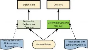
In this approach, alongside the (opaque) machine learning model used to predict the outcome we train another (not necessarily of the same type) to provide a set of reasons for the outcome. Because of the need for high performance (in providing an accurate explanation), this second model is also opaque. This ensemble is represented using the business decision modelling standard DMN, on the right.

DMN DRD Showing Two Model Ensemble: One Model Explains the Other

Both models are trained (in parallel) on sample data: the first labelled with the correct outcome and the second with the outcome and a supporting explanation. Then we apply both models in parallel: one provides the outcome and the other the explanation. This approach has some important drawbacks in practice:

• It can be very labour intensive to train the explanation model because you cannot reply on historical data (e.g. a history of who defaulted on their loans) for the explanation labels. Frequently you must create these labels by hand.
• It is difficult to be sure that your explanation training set has full coverage of all scenarios for which explanations may be required in future.
• You have no guarantee that the outcome of the first model will always be consistent with that of the second. It’s possible, if you are near the decision boundary, that you might obtain a loan rejection outcome from the first model and a set of reasons for acceptance from the second. The likelihood of this can be reduced (by using an ensemble) but never eliminated.
• The explanation outputs stand alone and no further explanation is available because the model that produced them is itself opaque.
• The two models are still opaque, so there is still no general understanding of how they work outside the outcome of specific cases.

Value Perturbation

This approach uses a system like LIME to perturb the features of inputs to an opaque AI model to see which ones make a difference in the outcome (i.e., cause it to cross a decision boundary). LIME will ‘explain’ an observation by perturbing the inputs for that observation a number of times, predicting the perturbed observations and fitting an explainable model to that new sample space. The idea is to fit a simple model in the neighbourhood of the observation to be explained. A DMN diagram depicting this approach is shown below.

DMN DRD Showing How LIME Produces Explanations for Opaque AI Modules

In our loan example, this technique might reveal that, although the loan was rejected, if the applicant’s house had been worth $50000 more or their conviction for car-theft was spent they would have been granted the loan. This technique can also tell us which features had very limited or no impact on the outcome.

This technique is powerful because it applies equally to any predictive machine learning model and does not require the training of another model. However it has a few disadvantages:

• Each case fed to the machine learning model, must be replicated with perturbations to every feature (attribute) in order to test their significance so the input data volume to the machine learning model (and therefore the cost of using it) rises enormously.
• As above, the model is still opaque, so there is still no general understanding of it works outside the outcome of specific cases
• As pointed out in the original paper on LIME, It relies on the decision boundary around the point of interest being a good fit with the transparent model. This may not always be the case, so, to combat this, a measure of the faithfulness of the fit is produced.

Using an Ensemble

The use of multiple machine learning models in collaborating groups (ensembles) has been common practice for many decades. The aim of bagging (one popular ensemble technique) is typically to increase the accuracy of the overall model by training many different sub-models on the same data so they each rely on different quirks of that data. This is rather like the ‘wisdom of crowds’ idea: one gets more accurate results if you ask many different people the same question because you accept their collective wisdom whilst ignoring individual idiosyncrasies. An ensemble of machine learning models is, collectively, less likely to overfit the training data. This technique is used to make random forests from decision trees. In use, the same data is applied to many models and they vote on the outcome.

This technique can be applied to solve transparency issues by combining a very accurate opaque model with a transparent model. Transparent models, such as decision trees generated by Quinlan’s C5.0, or rule sets created by algorithms like RIPPER (Repeated Incremental Pruning to Produce Error Reduction)[1], are typically less accurate than opaque alternatives but much easier to interpret. The comparatively poor performance of these transparent models (compared to the opaque ones) is not an issue because, over the entire dataset, the accuracy of an ensemble is usually higher than that of the best member providing the members are sufficiently diverse. A DMN model explaining this approach is shown below.

DMN DRD Showing Ensemble of Opaque and Transparent AI Modules

However the real advantage of this approach over the others is that because the transparent models are decision trees, rules or linear models they can be represented statically by a decision service. In other words, the decision tree or rules produced by the transparent analytic can be represented directly in DMN and made available to all stakeholders. This means that this approach not only provides an explanation for any outcome, but also an understanding (albeit an approximation) of how the decision is made in general, irrespective of any specific input data.

Using Ensembles in Practice

The real purpose of these transparent models is to produce an outcome and an explanation. Clearly the explanation is only useful if the outcome of the transparent and opaque models agree for the data provided. This checking is the job of the top level decision in the DRD shown. For each case there are two possibilities:

• The outcomes agree, in which case the explanation is a plausible account of how the decision was reached (note that it is not necessarily ‘the’ explanation as it has been produced by another model).
• The outcomes disagree, in which case the explanation is useless and the outcome is possibly marginal. In a small subset of these cases (when using techniques like soft voting) the transparent model’s outcome may be correct making the explanation useful. Nevertheless the overall confidence in the outcome is reduced because of the split vote.

The advantages of this approach is the fact that we have a static representation of an opaque model in the DMN standard which gives an indication of how the model works and can be used to explain its behaviour both in specific cases and in general.

If the precision of our opaque model is 99% and that of our transparent model is 90% (figures obtained from real examples) then the worst case probability for obtaining an accurate outcome and a plausible explanation is 89%. Having a parallel array of transparent decision models would increase this accuracy at the cost of making the whole model harder to understand. Individual explanations would retain their transparency.

Explanation Based Prediction

This is a relatively new approach typified by examples like CEN (contextual explanation networks) in which explanations are created as part of the prediction process without overhead. This is a probabilistic, graph based approach based on neural networks. As far as we are aware there are no generally-available implementations yet. The key advantages of this approach are:

• The explanation is, by definition, an exact explanation of which a given case yielded the outcome it did. None of the other approaches can be sure of this.
• The time and accuracy performance of the predictor is broadly consistent with other neural networks of this kind. There are no accuracy or rum-time consequences for using this approach.

The disadvantages with this approach is that it only works with a specific implementation of neural networks (which is not yet generally supported) and only yields a case-by-case explanation, rather than a static overview of decision-making.

Conclusion

Decision Modelling is an invaluable way of improving the transparency of certain types of narrow AI modules, machine learning models and predictive analytics which are almost always non-transparent (opaque). A particularly powerful means of doing this for datasets with fewer than 50 features is to combine both opaque and transparent predictors in an ensemble. The ensemble can then provide both an explanation for the outcome of a specific case and a general overview of the decision making process.

The transparent model uses a decision tree or rules to represent the logic of classification. Using DMN to represent these rules provides a standard and powerful means of making the model transparent to many stakeholders. DMN can also be used to represent the ensemble itself as shown in the articles’ examples.

Dr Jan Purchase and David Petchey are presenting two examples of this approach at Decision CAMP 2018 in Luxembourg, 17-19 September 2018. Why not join us?

Acknowledgements

My thanks to David Petchey for his considerable contributions to this article. Thanks also to CCRI for the headline image.

[1] Repeated Incremental Pruning to Produce Error Reduction (RIPPER) was proposed by William W. Cohen as an optimized version of IREP. See William W. Cohen: Fast Effective Rule Induction. In: Twelfth International Conference on Machine Learning, 115-123, 1995.

[2] Contextual Explanation Networks Maruan Al-Shedivat, Avinava Debey, Eric P. Xing, Carnegie Mellon University, January 2018.