Automated Structural Analysis of Electric Poles using AI and Computer Vision
Blog: Indium Software - Big Data
Recently, we have been working with a global construction and engineering consulting firm that provides technology-enabled solutions to the power, oil & gas, environmental and real estate sectors. We are building AI based solutions for them for multiple use-cases, leveraging our experience in NLP, Computer Vision and structured data analysis.
One of these use-cases involves extracting structural information from photos of electric poles. This includes first identifying the type of pole I.e., single-phase or three-phase, and then spotting the supply space and communication space as distinct zones in the pole. After that, the equipment and wires in the two zones would be detected separately. It is also particularly useful in a lot of applications to estimate the direction the wires are headed in terms of the four cardinal directions.
You might be interested in: Text Extraction And The Role It Plays In Digital Transformation
In this writeup, we will describe how we were able to extract the structural information using a combination of popular deep learning models and novel custom algorithms.
To get your unstructured data extracted, classified or summarized in a cost effective and fast way, Get in touch with us:
Contact us now!
Pole type Classification
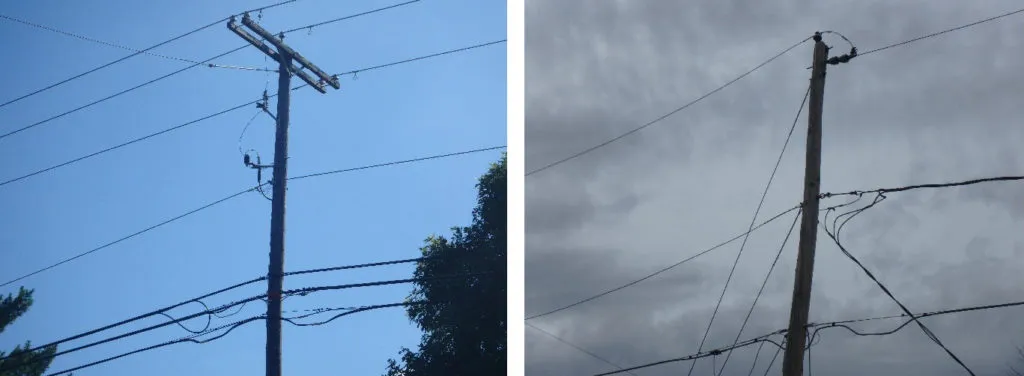
Electric poles can be broadly classified into two types – single phase and three phase poles. Structurally, three phase poles chiefly differ from single phase poles in that they have cross arm object(s) at the top of the pole. A couple of examples of both can be seen in Fig 1.
To perform this classification automatically, we used VGG16 pretrained deep-learning model with imagenet weights and trained the deep learning model for 30 epochs. A total of over 8000 annotated pole images were used in this training. After training, the model gave 90% accuracy on unseen test samples.

Detecting Equipment
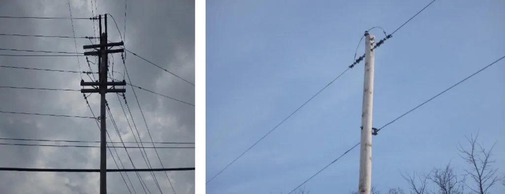
Equipment detection involved identifying various objects in the pole images (except wires). There were 15 categories of objects of interest including transformers, street lights and wireless antennas.
GCP Object Detection was used to solve this problem. After training for 25 node hours, the model was able to achieve a precision of 88.8% and a recall of 72% on test data.
Detecting Wires
After equipment, the major problem at our hand is wire detection. We modeled the wire detection to be an instance segmentation problem. Instance segmentation is an approach that identifies, for every pixel, a belonging instance of the object. It differs from related semantic segmentation in that it detects each distinct object of interest in the image as separate instances.
We used Facebook’s state-of-the-art instance segmentation model to do this. It is called Detectron2, is written in PyTorch and is hugely popular.
Hundreds of images were annotated for wires using the open source Labelme software. The annotations were converted to COCO format using scripts given along with the Labelme package. Detectron2 was then trained on these images for only a few epochs. Unlike other instance segmentation models like Mask-RCNN, Detectron2 takes much lesser iterations to get trained. The whole training on this reasonably big dataset of ~2500 images took only half an hour with Detectron2.
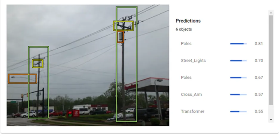
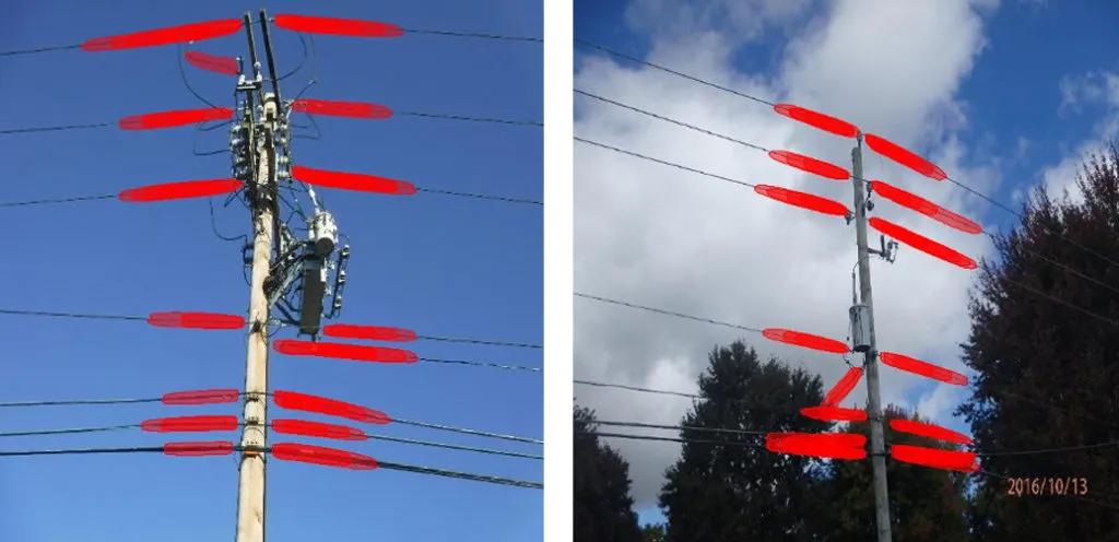
After training, the model was able to detect all the wires present in the image. The accuracy is quite good, and there were only a few images where it missed some wires. Some sample outputs are shown in Fig 3.
Classifying Wires
Once the wires are detected, we can classify them into supply or communication depending on where they lie with respect to the pole. The communication and supply zone masks are obtained independently by training another Detectron2 model. Here, the annotations were the boundaries of the two zones, instead of wires. Training procedure was otherwise identical to wire detection case.
With this model, we could classify each wire into either of these categories depending on the distance between the wire and zone mask.
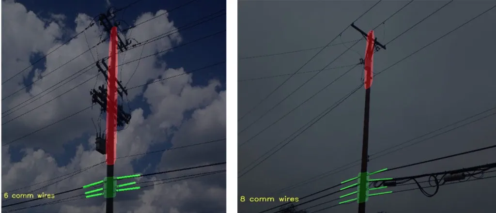
There was interest in particular, in capturing the number of communication wires. This was because we already had an idea about the supply space as to whether it is three-phase or single-phase, but no information on the communication space. So we wrote a pipeline to process the image and return a count of number of communication wires present in it. This involved OpenCV second level processing of the Detectron2 outputs as explained below:
- Some post processing of wires outputs:
- The left most point and right most point of each wire is identified and each wire is considered as a straight line segment between the points
- Wires that intersect, or are too close to another, or have a high overlap with other wires, or are too far from the pole are left out of analysis
- The communication space and supply space for each image is converted into contours i.e. taking only the boundary points of the masks.
- The distance between every pair of zone boundary point and wire endpoint is calculated. If the minimum of all these occurs with the communication mask, then that wire is taken as a communication wire and marked in green.
Some of the outputs of this pipeline are shown in Fig 4
Estimating wire direction (Three phase poles)
For wire direction, we came up with two separate approaches to tackle single phase and three phase poles. Three phase poles chiefly differ from single phase poles in that they have cross arm(s) usually at the top of the pole.
The length of cross arm varies from maximum when we view the pole from a far off point, looking at it parallel to the wires. It starts decreasing as we walk towards the pole parallel to the wires, and reaches zero when the view is perpendicular. It starts increasing again as we walk away from the pole in the back spans. This variation could be used to model the viewing direction as a function of cross arm length. For simplicity, we assume a linear relationship between the two.
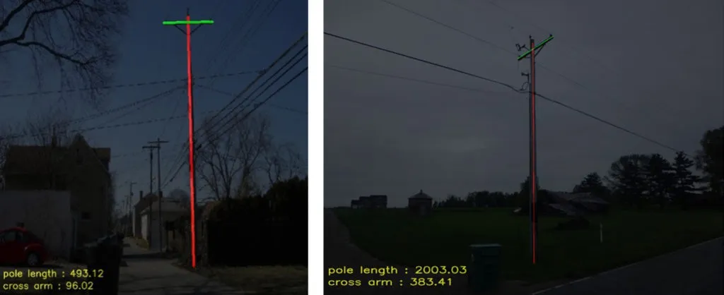
Like before, the pole and cross arm objects and their corresponding lengths can be computed using Detectron2 first and OpenCV post processing afterwards. The normalized cross arm length is defined as the ratio between cross arm length and pole length. This measure is expected to be more robust to variations in positions while clicking the photos.
Photos we deal with come with GPS information loaded as metadata. This is called the EXIF data of the file, and can be extracted using libraries like GPSPhoto in Python. Out of this information, we will be using the camera facing direction value that was captured by the compass in the camera. It comes as a value between 0 and 360 with 0 referring to true North, and other values referring to the displacement clockwise from North.
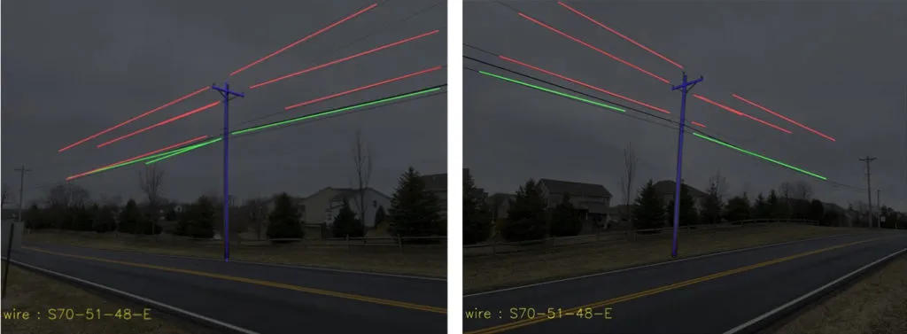
Now if we are given two photos of poles with the GPS facing direction and the normalized cross arm lengths computed, we can fit a line between these two photos’ sample points. We then predict the value of the facing direction when the cross arm length is exactly zero. This is the perpendicular view direction of the pole. Adding 90⁰ to this value gives the direction of the wires, because the principal wires are approximately normal to the pole at the point of intersection.
This algorithm works quite well in practice when we test it on some images captured from the field. The algorithm is further illustrated in Fig 5 and 6.
Estimating wire direction for Single phase poles
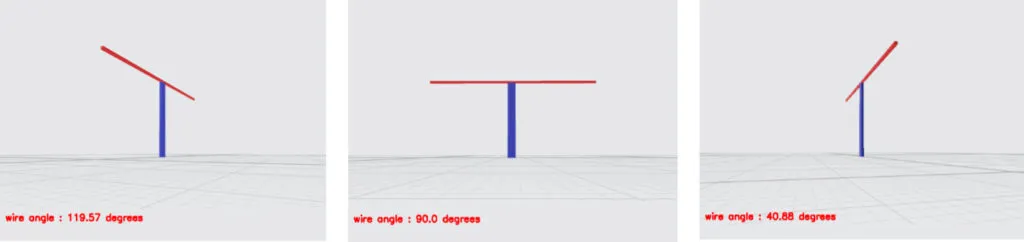
Single phase poles don’t have cross-arm objects, so the above approach can’t be used here. We found a way through this using the angle between the top most wire and the pole. This angle, like the normalized cross arm length can be assumed to linearly vary with the camera viewing angle.
For consistency, we always measure only the third quadrant angle (at the left bottom) with respect the wire and pole segments. The measurement itself can be easily done with Python assuming the wire and pole to be both vectors.
From two images clicked from the same side of the pole, a linear model can be fit and prediction for wire direction got, just like the three-phase case. If more images are given, we can fit a linear regression model. We see in Fig 8 that the values of these regression models on field data are quite good, providing validation for the approach.
But one thing while dealing with images clicked around the single phase pole is that we need to apply a correction when the viewer crosses over from one side to another perpendicular to wire direction. This correction might not always work and can lead to spurious samples, so it is best to avoid this kind of a cross-over while shooting photos of poles.
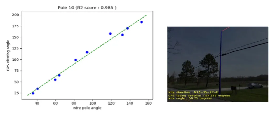
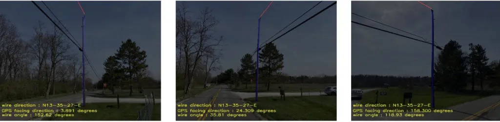
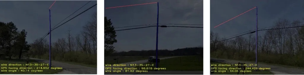
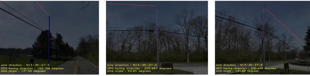
value of the fit provides validation for the modeling. The remaining ten images show the objects (pole in blue and top most wire in red) used to calculate the wire-pole angle. The estimated direction of N12-36-27-E is computed from the regression fit, and is written to the bottom of each of the contributing pole images.
Summary
We saw how AI and deep learning can give useful structural information from photos of electric poles. We used VGG16 to classify the pole as single-phase or three-phase. We then used GCP Object Detection to detect a variety of equipment in electric pole photos.
We saw that Detectron2 is a powerful instance segmentation model capable of adapting to multiple problem cases. We used it for detecting all the wires in the image. We also used it for pole zone segmentation to classify the wires into two categories and for cross-arm length computation.
We further showed how to predict the direction of the wires from coupling the objects detected in these images with GPS information embedded in the photo. The accuracy of both the direction algorithms (single-phase and three-phase) is good on unseen test samples, providing proof for the veracity of the modeling approach.
While we have focused on the wire and electric pole problem, these techniques are universal. They can be easily extended to other domains with just a few tweaks.
The post Automated Structural Analysis of Electric Poles using AI and Computer Vision appeared first on Indium Software.